Cloud‑Native Pipelines for Scientific Data Processing with Prefect and Dask

Introduction

The aim of this article is to provide an extended tutorial on the open-source libraries that we use to build the OceanStream cloud‑native data processing stack used to ingest data from sonar instruments and other marine sensors. We will describe the general principles of cloud‑native formats, introduce the Zarr storage format for multidimensional arrays, explain how tools like xarray and echopype work with data stored using the Zarr format, discuss Dask and its concept of chunking, and finally show how Prefect 3 orchestrates complex data workflows. 

Even though the examples are tailored for our use-case (hydroacoustics), they are applicable to any domain that works with large multidimensional datasets. Familiarity with Python programming some knowledge of data analysis libraries and concepts (e.g. NumPy, pandas, Jupyter notebooks) is assumed.

Why cloud-native?

Traditionally, scientific data is stored in formats like NetCDF or HDF, which are designed for local storage and access as sequential reads. But over the past few decades, recent advances in hardware and instrument design have led to a dramatic increase in data volume which often makes it inefficient and often impractical to continue working using a local desktop machine. In oceanography and hydroacoustics in particular, high resolution echosounders like the EK80 produce raw data files that can be several gigabytes in size for just a few hours of data collection.

At the same time, cloud computing has introduced object storage systems and protocols that are optimized for storing and accessing large amounts of data in a distributed and non-sequential manner. This has led to the development of new data formats and tools that are designed to work with cloud storage systems, such as Zarr and the Pangeo family.

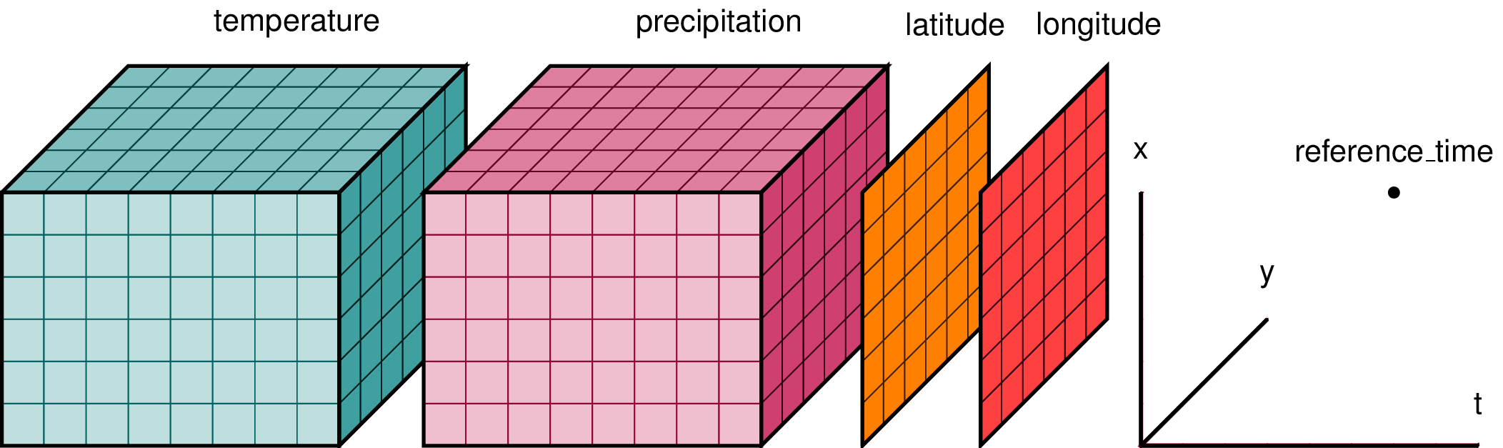
High resolution data in oceanography or climate sciences is often multi‑dimensional arrays of measurements over time and space – for example, 3D sonar backscatter arrays across frequencies, ping number and range, or 4D climate model outputs across longitude, latitude, depth and time.

Cloud-native means that working with this kind of data can be done in way that doesn't require downloading gigabytes (often terabytes) to your local machine. Instead, you can work directly with data from cloud object storage (such as S3, GCS or Azure Blob Storage) using tools that are optimised for this kind of access pattern, such as xarray and Dask.

Cloud‑native data formats

Traditional file formats such as CSV or classical NetCDF are designed to be written to and read from local disks. When these files are placed in object storage (e.g., Amazon S3 or Azure Blob Storage) they cannot be accessed efficiently because retrieving a small subset of the data requires downloading the entire file.

In contrast, cloud‑native (or cloud‑optimized) formats are specifically designed for remote object storage. Cloud‑native formats allow partial and parallel reads, enable metadata to be fetched in a single HTTP request, expose small addressable chunks via files or internal tiles, and integrate with high‑level analysis libraries and distributed frameworks.

Datasets stored in cloud-native formats are accessible over HTTP using range requests, which is essential because latency is high when retrieving data over the internet. So data is organised into chunks and metadata is easy to fetch, enabling clients to read only the required portions of a dataset and in a concurrent manner.

The Zarr format

Zarr is an open, community‑maintained format for storing chunked, compressed N‑dimensional arrays. Each array is divided into chunks and stored in a key–value store; the keys are the chunk indices and the values are binary files containing compressed array blocks.

The Zarr specification states that a dataset consists of one or more groups and arrays, with associated attributes. Each chunk of an array is stored in its own object, which can be accessed independently.

This design enables parallel read/write operations because different processes can work on different chunks concurrently. Zarr stores can live in memory, on disk, inside ZIP files, or in remote object stores like Amazon S3 and Azure Blob Storage.

Zarr organizes metadata and data as files within a directory (or “bucket” in cloud storage). At the top level, a .zgroup JSON file defines the group and lists its child arrays or groups. Each array resides in its own subdirectory containing a .zarray JSON file specifying the data type, shape, chunk sizes, compression settings and fill values. Array attributes are stored in .zattrs. Under the array directory, each chunk is saved as a file whose name encodes its chunk indices (e.g., 0.0, 1.0, 2.1).

The figure above illustrates this structure: a zgroup defines the root group; inside an array’s folder the .zarray file describes the array metadata; .zattrs holds user‑defined attributes; and numeric files represent compressed chunks. Because the index is separate from the data, a client can read the metadata file in one request and then fetch only the needed chunks.

xarray: labeled arrays for scientific data

xarray is an open-source library developed by the same group that defined the Zarr format, and, building upon the NetCDF data model, provides labeled N‑dimensional arrays with coordinates and attributes. It is also part of the  Pangeo ecosystem.

The core data structures are DataArray (a single N‑D array with named dimensions and coordinates) and Dataset (a dict‑like container of multiple DataArray objects). Xarray adds labels–dimension names, coordinate arrays and metadata–to raw NumPy arrays so that operations can be expressed by name rather than by index. For example, you can select a subset of data by specifying dataset.sel(time='2025-09-15', depth=slice(0,50)) instead of calculating index positions manually.

Xarray supports operations such as arithmetic, reductions, broadcasting, groupby, resampling and merging; these operations propagate coordinate information and attributes. Because xarray follows the NetCDF data model, it can read and write NetCDF, HDF5 and GRIB files. More importantly for cloud workflows, xarray integrates very well with Zarr: opening a Zarr store using xr.open_zarr() returns a lazy Dask array if Dask is available.

Lazy arrays delay computation until explicitly invoked by .compute(), enabling you to compose complex analyses without loading all data into memory.

Run an xarray/Zarr example

To run this example, you'll need to install the following dependencies:

# create a venv first
python3 -m venv .venv
source .venv/bin/activate

# install dependencies
pip install xarray zarr dask s3fs

Create a new xarray_zarr_demo.py file (or a new Jupyter notebook, if we prefer that instead).

import xarray as xr
import numpy as np
import zarr

# Create a small example dataset and write with a chunking strategy
time = np.arange(0, 3600, 1)  # seconds
range_bin = np.arange(0, 1800, 1)  # samples

ds = xr.Dataset(
    data_vars=dict(
        Sv=(["time", "range_bin"], np.random.randn(time.size, range_bin.size).astype("float32")),
    ),
    coords=dict(time=("time", time), range_bin=("range_bin", range_bin)),
    attrs={"convention": "SONAR-netCDF4-like (illustrative)"},
)

# chunk sizes should reflect read patterns (time-scan, or depth stripes, etc.)
ds_chunked = ds.chunk({"time": 300, "range_bin": 256})

# Write to a local Zarr store
out = "sonar_scan.zarr"
ds_chunked.to_zarr(out, mode="w")

# Lazy open without loading into memory
ds2 = xr.open_zarr(out)

Here's the ds dataset we created:

<xarray.Dataset> Size: 26MB
Dimensions:    (time: 3600, range_bin: 1800)
Coordinates:
  * time       (time) int64 29kB 0 1 2 3 4 5 6 ... 3594 3595 3596 3597 3598 3599
  * range_bin  (range_bin) int64 14kB 0 1 2 3 4 5 ... 1795 1796 1797 1798 1799
Data variables:
    Sv         (time, range_bin) float32 26MB 0.7469 1.758 ... -0.5222 -0.6784
Attributes:
    convention:  SONAR-netCDF4 v1.0

And for more context, the chunked ds_chunked dataset:

<xarray.Dataset> Size: 26MB
Dimensions:    (time: 3600, range_bin: 1800)
Coordinates:
  * time       (time) int64 29kB 0 1 2 3 4 5 6 ... 3594 3595 3596 3597 3598 3599
  * range_bin  (range_bin) int64 14kB 0 1 2 3 4 5 ... 1795 1796 1797 1798 1799
Data variables:
    Sv         (time, range_bin) float32 26MB dask.array<chunksize=(300, 256), meta=np.ndarray>
Attributes:
    convention:  SONAR-netCDF4 v1.0

Save the Zarr store to Amazon S3

And now for something completely different, we will save our example dataset to the cloud – the Amazon AWS cloud that is.

First we will have take care of the preliminaries, like creating an account and an S3 bucket. This article assumes that you are entirely new to AWS and do not have an account.

Create a free AWS account

Go to https://aws.amazon.com and complete the sign-up process (shouldn't take more than 10 minutes).

Then install the aws CLI (required for this tutorial): https://docs.aws.amazon.com/cli/latest/userguide/getting-started-install.html

Once you are logged in to the AWS Console, create a access key, then open a new Terminal/CMD window and run the following:

aws configure

This should prompt you to enter the AWS credentials, region, and output format.

AWS Access Key ID: 
AWS Secret Access Key: 
Default region name [eu-central-1]: 
Default output format [json]: 

Create a new S3 bucket with anonymous access

For this tutorial, we'll create an anonymous S3 bucket to make it easier to run the xarray demo, but for your own data you should of course use proper authentication credentials.

Run the following commands to create a new S3 bucket called xarray-zarr-demo:

aws s3 mb s3://xarray-zarr-demo

aws s3api put-public-access-block \
  --bucket xarray-zarr-demo \ 
  --public-access-block-configuration "BlockPublicAcls=false,IgnorePublicAcls=false,BlockPublicPolicy=false,RestrictPublicBuckets=false"

aws s3api put-public-access-block \
  --bucket xarray-zarr-demo \
  --public-access-block-configuration '{
    "BlockPublicAcls": false,
    "IgnorePublicAcls": false,
    "BlockPublicPolicy": false,
    "RestrictPublicBuckets": false
  }'

Save the dataset to the S3 Zarr store

Now that the S3 bucket is created using public anonymous access, we can simply use it in our code without any other steps.

Add the following lines at the end of the xarray_zarr_demo.py:

# Save the chunked dataset to the S3 bucket
ds_chunked.to_zarr("s3://xarray-zarr-demo/sonar_scan.zarr",
           mode="w",
           consolidated=True,
           zarr_format=2)

# load directly from S3
ds_from_s3 = xr.open_zarr("s3://xarray-zarr-demo/sonar_scan.zarr")

You can also load just a subset of the data, using an index-based window:

ds_from_s3 = xr.open_zarr("s3://xarray-zarr-demo/sonar_scan.zarr")

# index-based window
subset = ds2["Sv"].isel(time=slice(600, 1200), range_bin=slice(0, 512)).load()

For more info on xarray indexing, check out the docs: https://docs.xarray.dev/en/latest/user-guide/indexing.html

Dask and Chunking

Dask is an open-source integrated library that offers a reliable way to distribute computations over several workers so processing can be parallelised.

At its core, Dask provides collections (arrays, dataframes, bags, and delayed objects) that mimic the interfaces of NumPy, pandas, and Python iterators but operate on-demand on many small pieces (known as chunks).

Dask coordinates many NumPy arrays arranged into chunks and supports a large subset of the NumPy API. It enables computations on arrays that are larger than memory by streaming data from disk and using blocked algorithms. This design allows Dask to utilise all CPU cores on a single machine and to scale across a cluster by scheduling tasks with the distributed scheduler.

In our previous example, dask is already used under the hood by xarray to do the chunking of the dataset. Dask takes care of loading only the chunks needed for a computation.

Running a Dask cluster

The simplest way to setup and use a Dask cluster is on your local machine, right in your script.

First install the additional dependencies:

# bokeh is optional, needed for the dask dashboard

pip install distributed "bokeh>=3.1.0" 

Update the previous Python script and add the following at the top:

from dask.distributed import LocalCluster

cluster = LocalCluster()          # Fully-featured local Dask cluster
client = cluster.get_client()

If you're using a Jupyter notebook, create a new cell and paste the code above.

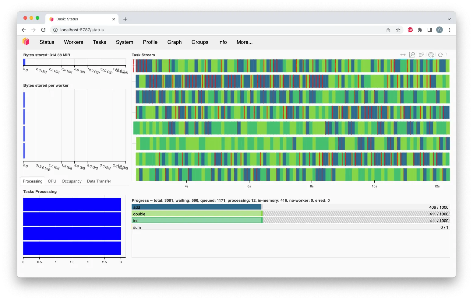
You'll also automatically get a dashboard running at http://127.0.0.1:8787/status

Orchestrating workflows with Prefect 3

Data processing pipelines involve many steps: downloading raw data, converting to Zarr, denoising signals, computing metrics, updating databases and notifying users. Prefect is an open‑source ETL (Extract-Transform-Load) Python framework for orchestrating these tasks.

Prefect organizes work into flows and tasks. A flow is a Python function decorated with @flow that defines the overall pipeline; a task is a function decorated with @task that encapsulates a unit of work. Flows can call tasks sequentially or conditionally, iterate over collections, and spawn subflows. Prefect keeps track of the state of each task (pending, running, succeeded, failed) and provides retries, caching and timeout mechanisms. Because tasks are plain Python functions, users can call third‑party libraries (e.g. xarray, echopype or Dask) directly within tasks.

Prefect supports several execution environments: tasks can run in a local process (ideal for development), in Dask clusters, in Kubernetes pods, or using serverless functions. Prefect also provides an implementation of workers for distributing the workflows and run them concurrently. It also integrates well with Dask via the prefect-dask package.

Installing Prefect 3

Simply run the following commands in your terminal (in the previously created venv virtual environment) to install Prefect, along with the Prefect Dask integration:

pip install prefect prefect-dask

Once the installation has finished, you can start the Prefect server to verify if it's working properly.

Run the following (use the background option):

prefect server start --background

This will automatically create a local SQLite database as well, which is fine for now. You can switch to a Postgres DB later. If everything went well, you should see the following output:

 ___ ___ ___ ___ ___ ___ _____
| _ \ _ \ __| __| __/ __|_   _|
|  _/   / _|| _|| _| (__  | |
|_| |_|_\___|_| |___\___| |_|

Configure Prefect to communicate with the server with:

    prefect config set PREFECT_API_URL=http://127.0.0.1:4200/api

View the API reference documentation at http://127.0.0.1:4200/docs

Check out the dashboard at http://127.0.0.1:4200

Also run the command to configure the server (make sure you're in the venv):

prefect config set PREFECT_API_URL=http://127.0.0.1:4200/api

Then you should be able to navigate to the dashboard at http://127.0.0.1:4200.

An end-to-end, cloud-native sonar data analysis pipeline

Now we're ready to proceed to the next stage in our tutorial, and implement a complete ETL processing pipeline in the Python libraries discussed thus far.

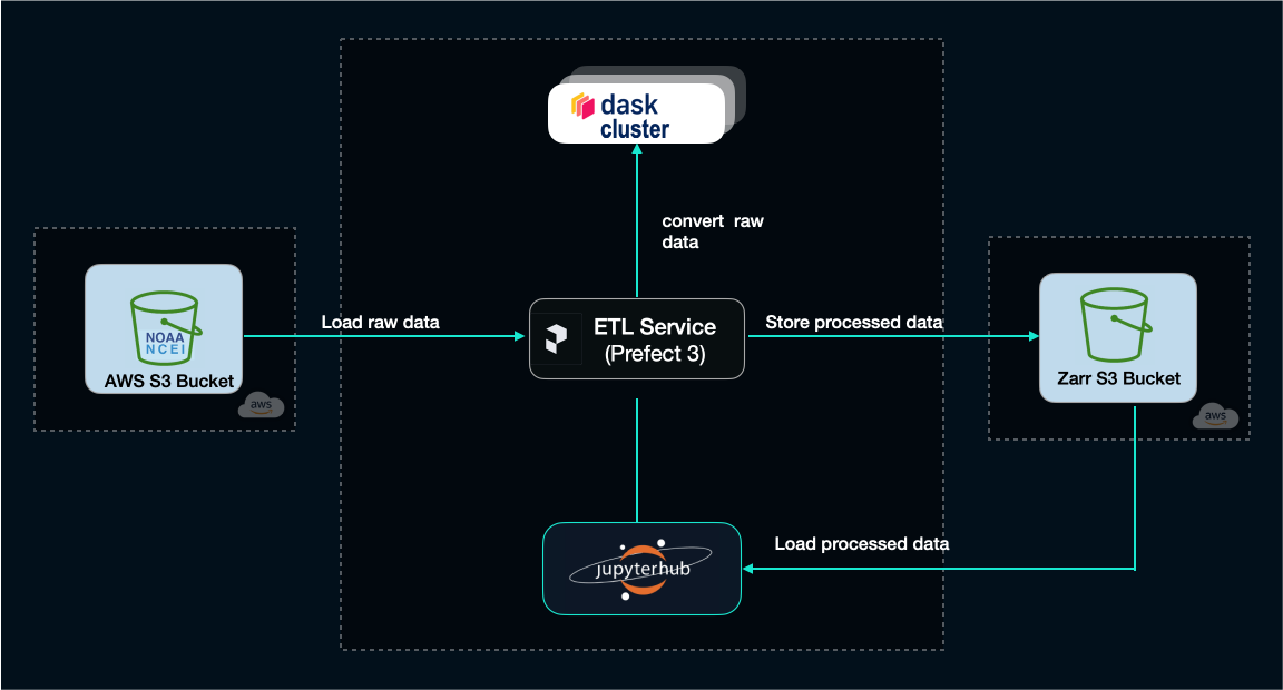
For our project we'll use some raw data from NOAA (National Oceanic and Atmospheric Administration). This is actual raw data collected during an oceanographic campaign in the North Atlantic using a narrow-band split-beam echosounder (EK60) – a type of sonar instrument used by marine scientists to collect hydroacoustic data from the water column, in order to study the marine life.

Here's the tasks we'll implement as Prefect flows:

1. we'll download a few raw files from one of these surveys from the NOAA S3 bucket
2. do some basic processing using the tools we've described so far
3. upload the processed result in a new S3 bucket that we'll create in our own AWS account

Learn more about the water column sonar data on this excellent NOAA article (you can also find more details and a map visualisation about the data we're using):

Download the raw data

We have a select only a very small subset of the entire raw data available from the survey – feel free to extend your dataset if you wish, there's plenty of data available in the public NOAA S3 bucket we have picked.

For this exercise, we want to demonstrate how to write a Prefect 3 flow which contains a basic task that download the raw data files onto your own local drive, and for this we need to introduce the concept of Prefect workers and work pools.

Create Prefect a work pool and local workers

There's several options for work pools, but we'll use the basic one that runs on our own machine: process.

Make sure the prefect server is running, under your existing venv and run the following command:

prefect work-pool create local-process --type process

This will create a new work pool called local-process. If successful, the output should be:

To start a worker for this work pool, run:

        prefect worker start --pool local-process

Now, we can go ahead and start 2 workers. Launch 2 separate terminals and run the command from the create work-pool output, making sure to activate the venv first.

# cd to the project directory and activate the venv
source .venv/bin/activate

# start a worker
prefect worker start --pool local-process

Output should be like:

Discovered type 'process' for work pool 'local-process'.
Worker 'ProcessWorker 0cbd2d83-f320-...' started!

Learn more about Prefect work pools on the Prefect docs: https://docs.prefect.io/v3/concepts/work-pools

Write the Prefect download-raw-data flow

Next, we'll write the actual Prefect flow and run it as a deployment. Wrapping it up as a Prefect deployment makes it easier to work with the flow, also from the Prefect UI, as we'll see in a bit.

Create a subfolder called prefect_flows in your project and create a new file download_raw_data.py, adding this content:

import logging
import sys
import httpx
from pathlib import Path
from prefect import flow, task
from prefect.task_runners import ThreadPoolTaskRunner


DEST_FOLDER = Path("../raw_data")
BUCKET_URL = "https://noaa-wcsd-pds.s3.amazonaws.com"
PREFIX = "data/raw/Henry_B._Bigelow/HB1907/EK60"
FILENAMES = [
    "D20190727-T035511.raw",
    "D20190727-T042803.raw",
    "D20190727-T050056.raw",
    "D20190727-T053138.raw",
    "D20190727-T060130.raw"
]


@task(
    retries=5,
    retry_delay_seconds=30,
    task_run_name="download-file-{file_name}",
)
def download_file(url: str, download_dir: str, file_name: str) -> str:
    print(f"Starting download of {file_name} from {url}...")
    dest = Path(download_dir) / url.rsplit("/", 1)[-1]
    dest.parent.mkdir(parents=True, exist_ok=True)

    with httpx.stream("GET", url, timeout=None) as r:
        r.raise_for_status()
        with dest.open("wb") as f:
            for chunk in r.iter_bytes():
                f.write(chunk)

    print(f"Finished download of {file_name} to {dest}")

    return str(dest)


@flow(
    name="download-raw-data",
    task_runner=ThreadPoolTaskRunner(max_workers=2)
)
def download_raw_data(download_dir: str):
    task_futures = []

    for file_name in FILENAMES:
        url = f"{BUCKET_URL}/{PREFIX}/{file_name}"
        task_futures.append(download_file.submit(url=url, download_dir=download_dir, file_name=file_name))

    for future in task_futures:
        future.result()

    print("All files have been downloaded.")


if __name__ == "__main__":
    try:
        download_raw_data.serve(
            name='download-raw-data-from-noaa-s3',
            parameters={
                'download_dir': str(DEST_FOLDER)
            }
        )
    except Exception as e:
        logging.critical(f'Unhandled exception: {e}', exc_info=True)
        sys.exit(1)

We have picked only 5 raw files and set the max_workers to 2.

The next step now is to run the deployment which "serves" the flow. This will create a service locally that waits for triggers.

We'll keep it simple and run the deployment directly from the CLI, so make sure to open a new Terminal window and cd to the project. The Prefect server and workers should also be running at this point.

Run the following command:

# activate the venv first
source .venv/bin/activate

cd prefect_flows
python3 download_raw_data.py

This should output the following, which means that the flow is ready to be triggered:

Your flow 'download-raw-data' is being served and polling for scheduled runs!

To trigger a run for this flow, use the following command:

        $ prefect deployment run 'download-raw-data/download-raw-data-from-noaa-s3'

You can also run your flow via the Prefect UI: http://127.0.0.1:4200/deployments/deployment/1061e04c-7d78-4f7e-8f2d-eea01144b5b7

We'll go ahead and open the Prefect UI at http://127.0.0.1:4200/ and trigger a new run from there. Go to Deployments, navigate to our deployment (should be called "download-raw-data-from-noaa-s3") and click on the Run button in the top right corner, then "Quick run".

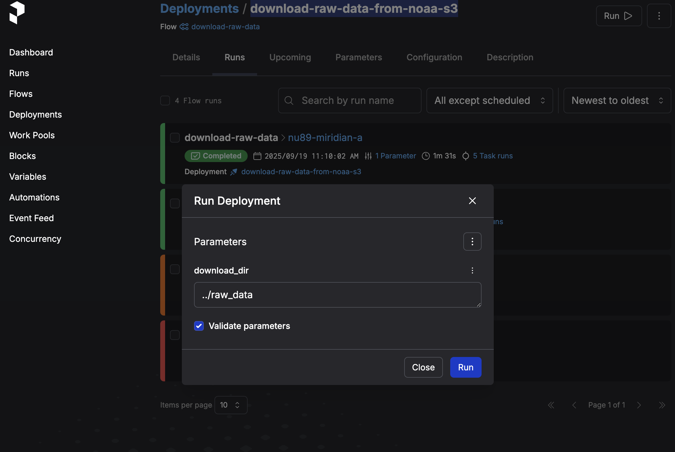
Now we can go ahead and run the flow, which will download the files. Prefect will show nice progress indicators for each task that's running.

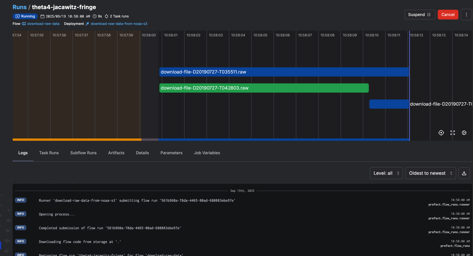
At the end of the flow run, you should have all the raw files in the raw_data subfolder.

Processing the raw data

Now we're ready to move on to the more complex part, which is also the more exciting and fun part. We'll write another similar Prefect flow which will convert the raw data into a standardised format and save it to Zarr, in an S3 bucket.

Write the Prefect convert-raw-data flow

In order to be able to efficiently work with the sonar data recorded in the raw files we've previously downloaded, we'll have to convert them using a specialised analysis tool.

The most popular and widely used Python open-source tool in hydroacoustic data analysis, and with a great documentation, is echopype. It has many of the most common features needed in the field for common tasks and computations, and for our tutorial it's an excellent fit.

Echoype uses xarray and Zarr behind the scenes so it integrates splendidly with our pipeline. Let's install it with:

# activate the venv if needed
source .venv/bin/activate

pip install echopype

Create a new convert_to_zarr.py file in the prefect_flows directory with the content below:

from pathlib import Path
from typing import Optional, Dict

from prefect import flow, task
from dask.distributed import LocalCluster
from prefect_dask import DaskTaskRunner
from prefect.futures import as_completed


DEFAULT_INPUT_DIR = Path("../raw_data")
S3_BUCKET_NAME = "xarray-zarr-demo"


@task(
    retries=3,
    retry_delay_seconds=60,
    task_run_name="convert-to-zarr-{raw_path}",
)
def convert_single_raw_to_zarr(
    raw_path: str,
    s3_bucket: str,
    s3_prefix: str = "",
    sonar_model: str = "EK60",
    overwrite: bool = True,
    storage_options: Optional[Dict] = None
) -> str:
    # Lazy import so workers don't need echopype at collection time
    import echopype as ep

    raw_path_p = Path(raw_path)
    if not raw_path_p.exists():
        raise FileNotFoundError(f"Input RAW file not found: {raw_path}")

    key_prefix = s3_prefix.strip("/")

    key = f"{key_prefix}/{raw_path_p.stem}.zarr" if key_prefix else f"{raw_path_p.stem}.zarr"
    zarr_uri = f"s3://{s3_bucket}/{key}"

    ed = ep.open_raw(str(raw_path_p), sonar_model=sonar_model)
    ed.to_zarr(zarr_uri, overwrite=overwrite, output_storage_options=storage_options)

    return zarr_uri


@flow(
    name="convert-raw-to-zarr",
    log_prints=True,
    task_runner=DaskTaskRunner(address="tcp://127.0.0.1:8786")
)
def convert_raw_to_zarr(
    input_dir: str,
    s3_bucket: str,
    s3_prefix: str = "",
    sonar_model: str = "EK60",
    overwrite: bool = True,
    glob_pattern: str = "*.raw",
    storage_options: Optional[Dict] = None
):
    input_path = Path(input_dir)
    if not input_path.exists():
        raise FileNotFoundError(f"Input directory not found: {input_dir}")

    raw_files = sorted(input_path.glob(glob_pattern))
    if not raw_files:
        print(f"No files matching '{glob_pattern}' found in {input_dir}.")
        return

    in_flight = []
    batch_size = 2

    for rp in raw_files:
        task = convert_single_raw_to_zarr.submit(
            raw_path=str(rp),
            s3_bucket=s3_bucket,
            s3_prefix=s3_prefix,
            sonar_model=sonar_model,
            overwrite=overwrite,
            storage_options=storage_options
        )
        in_flight.append(task)

        if len(in_flight) >= batch_size:
            finished = next(as_completed(in_flight))
            in_flight.remove(finished)

    for future_task in in_flight:
        future_task.result()


if __name__ == "__main__":
    cluster = LocalCluster(
        n_workers=2,
        scheduler_port=8786,
        threads_per_worker=1,
        memory_limit="8GB"
    )
    client = cluster.get_client()

    convert_raw_to_zarr.serve(
        name="convert-raw-to-zarr-serve",
        parameters={
            "input_dir": str(DEFAULT_INPUT_DIR),
            "s3_bucket": S3_BUCKET_NAME,
            "s3_prefix": "echodata",
            "sonar_model": "EK60",
            "overwrite": True,
            "glob_pattern": "*.raw",
            "storage_options": {}
        },
    )

Run and understand the convert-raw-data flow

Now that we have the new Prefect flow to convert the raw data files, we can run the file in the CLI to create a new deployment, similarly to how we've done it for the download raw data flow.

One important distinction: the convert-raw-data flow uses the DaskTaskRunner so we don't need to Prefect workers for this flow. We are creating a local Dask cluster which will manage its own workers:

cluster = LocalCluster(
    n_workers=2,
    scheduler_port=8786,
    threads_per_worker=1,
    memory_limit="8GB"
)

To activate the deployment, you simple run the following in your project folder:

# activate the venv first
source .venv/bin/activate

cd prefect_flows
python3 convert_to_zarr.py

Then, assuming you already downloaded the raw data using the previous flow, you can trigger the processing from the Prefect UI.

What the flow does

• convert_raw_to_zarr receives an input_dir and a glob_pattern (default *.raw) and enumerates the raw files found, and submits a task convert_single_raw_to_zarr to a worker
• inside the task, the echopype library is lazy-imported (imported inside the task) so just importing the module that defines the flow doesn’t require echopype on every machine. This also keeps “collection time” light on workers.
  • ep.open_raw(..., sonar_model="EK60") opens and decodes vendor RAW (EK60 by default) into an EchoData object. Echopype handles parsing, metadata, and calibration logic for you.
  • EchoData.to_zarr(...) writes a chunked, cloud-friendly Zarr store; we and construct a full s3://{bucket}/{key} URI and store the Zarr store directly in S3, using the same bucket xarray-zarr-demo from the previous example
  • You can also supply other bucket via the store_options parameter which will be forwarded echopype. You can pass credentials or flags here.
• Inside the flow, a manual in-flight cap (batch_size = 2) is implemented with as_completed: the loop submits tasks, keeps at most two running, and advances as each finishes. This is necessary because the DaskTaskRunner doesn't have max_workers parameter.

Which Prefect task runner to use?

The DaskTaskRunner we introduced here is very useful when you want to do more complex analysis where you'll to split the dataset in chunks and do the processing in parallel across multiple machines.

Of course, for processing a handful of raw data files, you can stick to the default ThreadPoolTaskRunner, which we could have done here. But I wanted to introduce the Dask concepts early on so we have a solid base for later tutorials where we'd do more memory and CPU intensive tasks, like computing the mean volume backscattering strength – a common task in hydroacoustics.

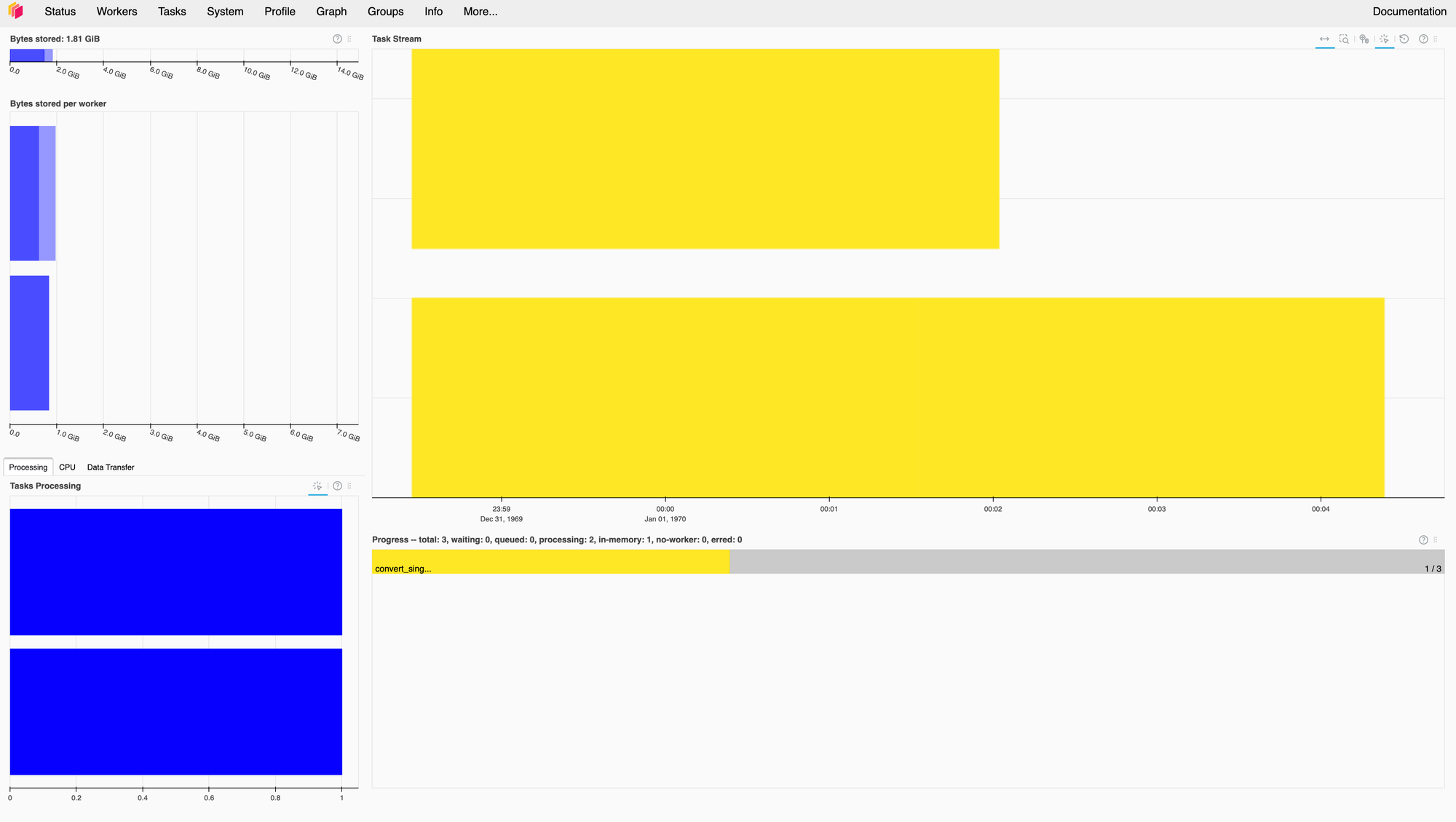
You can also use the Dask dashboard, which looks like this for our convert flow – not very sophisticated, but still...

Conclusion

Thanks for reading all the way here. You can find the code on Github – feel free to send PRs or requests for more prefect flows.

blog-tutorials-code/xarray-prefect-tutorial at main · OceanStreamIO/blog-tutorials-code

Contribute to OceanStreamIO/blog-tutorials-code development by creating an account on GitHub.

GitHubOceanStreamIO

If you want to get in touch with us, you can do so by writing us an email here: https://oceanstream.io/contact/