Plotting Sea‑Surface Temperatures Over the North-Atlantic using Cloud Optimised ERA5 Dataset

Climate and oceanographic analysis is often thought of as being performed on large scale super computers running in high performance computing clusters but, while that’s still true for many workloads, recently it has become more accessible to run some analyses by using cloud-optimised tools and datasets. In this article we will walk through a concrete example: calculating monthly Sea‑surface temperature (SST) statistics for the North Atlantic using the Analysis‑Ready, Cloud‑Optimised (ARCO) ERA5 dataset from ECMWF and visualising them on a map.

The workflow is implemented in Python and uses the xarray library for labelled multidimensional arrays and dask for parallel computation. The code is available as a Jupyter notebook on Github. The key tools we will use are xarray for manipulating labelled arrays and Dask for scaling computations – we've described these in detail in a separate tutorial: Cloud‑Native Pipelines for Scientific Data Processing with Prefect and Dask

Concretely, we'll do the following:

Connect to the ERA5 ARCO Zarr store hosted on Google Cloud.
Select a geographic subset covering the North Atlantic and nearby Arctic seas.
Use xarray and Dask to compute monthly SST fields lazily, streaming only the required chunks.
Render a high-resolution SST map with Cartopy and Matplotlib.

If you want to jump straight into the code, feel free to do so by grabbing the source code from here:

Analysis‑ready, cloud‑optimised (ARCO) datasets change the old paradigm of downloading gigabytes of NetCDF data and writing custom scripts to extract subsets by storing curated subsets of climate data in a cloud‑friendly, chunked format that can be streamed directly into analysis tools.

ERA5 and the ARCO initiative

ERA5 stands for ECMWF Reanalysis v5 – a state‑of‑the‑art meteorological reanalysis produced by the European Centre for Medium‑Range Weather Forecasts (ECMWF). Reanalysis datasets assimilate observations from satellites, weather stations and other platforms into a numerical model to generate a continuous, physically consistent record of the atmosphere, ocean and land surface.

The ARCO ERA5 project, led by Google Research and Google Cloud, makes this high‑resolution data easy to explore by storing it as cloud-optimised Zarr dataset. Unlike the traditional NetCDF files where each parameter and period is stored separately, the Zarr format groups related variables into classes (for example, model‑level wind, model‑level moisture, single‑level surface, reanalysis and forecast fields) and is optimised for cloud object storage.

The data are stored in chunks and the Zarr format allows tools like xarray to fetch only the relevant parts for a given query. This design enables efficient subsetting and streaming from cloud object storage; for example retrieving a long time series at a single location requires reading only the corresponding time slices rather than downloading complete global fields.

Set up the environment

In order to run this experiment locally in a Jupyter lab, we'll use Python along with the Xarray and Dask libraries to access remote data and perform chunked calculations. The Xarray API allows us to open multidimensional arrays stored in cloud-optimised formats like Zarr and to manipulate them using familiar pandas‑like semantics. Dask parallelises operations across multiple cores and orchestrates I/O so that only the data needed for each computation are loaded into memory.

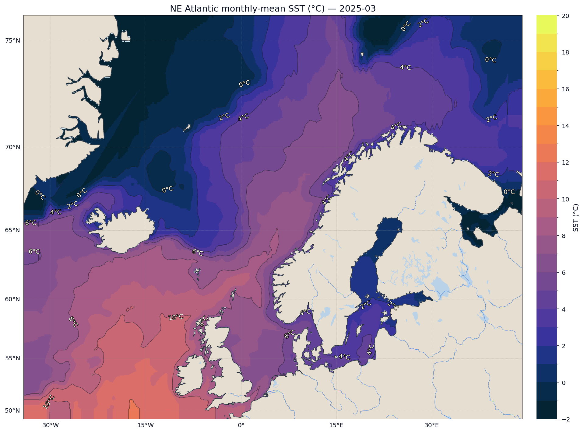
For our task, we'll compute sea‑surface temperature (SST) in the North Atlantic and Norwegian Sea. SST is a key indicator in climate and oceanographic research for understanding things like heat transport into northern Europe and the Arctic, the growth of sea ice, regional weather patterns, and the distribution of marine pelagic life.

First, install the requirements with:

pip install "xarray[complete]" dask[complete] gcsfs cartopy matplotlib numpy

Load the Zarr Dataset from Google Cloud

First we create a local Dask cluster. By default the cluster will start one worker per available CPU, but we limit each worker to a single thread to avoid Python’s Global Interpreter Lock (GIL). We also instruct xarray to split large chunks when slicing arrays.

The following code sets up the cluster and opens the ARCO Zarr store:

import numpy as np
import xarray as xr
import os
import dask
from dask.distributed import Client, LocalCluster


# Path to the ARCO ERA5 Analysis‑Ready 0.25° Zarr store
zarr_path = "gs://gcp-public-data-arco-era5/co/single-level-reanalysis.zarr-v2"

cluster = LocalCluster(
    n_workers=max(1, os.cpu_count() - 1),
    threads_per_worker=1,           # avoid GIL thrash for Python-level ops
    processes=True,
    memory_limit="auto"
)
client = Client(cluster)

# Make xarray use Dask by default
dask.config.set({"array.slicing.split_large_chunks": True})

ds = xr.open_zarr(
    zarr_path,
    chunks={},
    storage_options={"token": "anon"},
)

The storage_options parameter specifies anonymous access because the bucket is public. Xarray returns lazy Dask arrays for each variable; no data are downloaded until we actually compute or inspect them.

Define and subset a region of interest

Our goal is to analyse SST around Scandinavia and the adjacent North Atlantic. We define a bounding box that covers Iceland, the Norwegian and Barents Seas, parts of Greenland and extends far north toward the Arctic.

The coordinates are given as (lon_min, lon_max, lat_min, lat_max). The notebook uses the following values:

# Iceland + Norwegian/Barents, a touch of Greenland, farther north
TARGET_EXTENT = (-32.0, 42.0, 50.0, 84.0)  # (lon_min, lon_max, lat_min, lat_max)

if lon_name not in ds.coords or lat_name not in ds.coords:
    raise KeyError(f"Could not find lon/lat coords. Found coords: {list(ds.coords)}")

# Normalize once on the dataset coordinate (lazy; no load)
ds = ds.assign_coords({lon_name: ((ds[lon_name] + 180) % 360) - 180})

# Load coord arrays into NumPy to build a deterministic bbox index
lon_np = ds[lon_name].load().values
lat_np = ds[lat_name].load().values

# Build bbox mask from TARGET_EXTENT
lon_min, lon_max, lat_min, lat_max = TARGET_EXTENT
bbox_mask_np = (
    (lon_np >= lon_min) & (lon_np <= lon_max) &
    (lat_np >= lat_min) & (lat_np <= lat_max)
)
bbox_idx = np.where(bbox_mask_np)[0]
if bbox_idx.size == 0:
    raise ValueError(f"No points found inside bbox {TARGET_EXTENT}. "
                     "Check longitude normalization and bounds.")

# Subset main dataset by NUMERIC indices (keeps lon/lat/value alignment)
region_ds = ds.isel({spatial_dim: bbox_idx})

sst = region_ds["sst"]
ci = region_ds["siconc"]

# Convert to Celsius and mask sea-ice (>= 0.15)
sst_C = (sst - 273.15).astype('float32').rename("sst_C")
sst_C = sst_C.chunk({"time": 12, spatial_dim: "auto"})

ice_threshold = 0.15

if ci is not None:
    sst_C = sst_C.where(ci <= ice_threshold)

lon_arr = region_ds[lon_name].values
lat_arr = region_ds[lat_name].values

valid = np.isfinite(lon_arr) & np.isfinite(lat_arr)
if not np.any(valid):
    raise ValueError("No finite lon/lat points in region_ds to compute plot extent.")

xmin = float(np.nanmin(lon_arr[valid])); xmax = float(np.nanmax(lon_arr[valid]))
ymin = float(np.nanmin(lat_arr[valid])); ymax = float(np.nanmax(lat_arr[valid]))

# Padding in degrees (small but avoids tight clipping)
pad_x = max(0.75, 0.03 * (xmax - xmin))
pad_y = max(0.60, 0.03 * (ymax - ymin))

# Optional cap to avoid extreme Mercator stretch at very high latitudes
CAP_NORTH = 76.0  # set to None to disable

xmin = max(-180.0, xmin - pad_x)
xmax = min( 180.0, xmax + pad_x)
ymin = max( -90.0,  ymin - pad_y)
ymax = min((CAP_NORTH if CAP_NORTH is not None else 85.0), ymax + pad_y)

plot_extent = [xmin, xmax, ymin, ymax]

# Monthly mean SST
sst_monthly = sst_C.resample(time="1MS").mean()

We construct a boolean mask to select only those indices within our bounding box and then we use the .isel method with integer indices to avoid Dask evaluating the entire coordinate arrays when building a boolean mask lazily.

The sst variable is stored in Kelvin, so we subtract 273.15 to convert to degrees Celsius and rename it. The sea‑ice concentration variable siconc is used to mask grid points where ice coverage exceeds 15%, a common threshold distinguishing open water from ice. If siconc is not present, the masking is skipped.

Then we re-chunk the sst_C array along time and the spatial dimension. Resampling to daily or monthly means requires reading across time, so smaller time chunks (e.g. 12 hour slices) help reduce memory consumption.

This step takes about 10 minutes on my Macbook Pro (M1, 2021, 32Gb RAM), so you'll have to be a bit patient.

Plot the sea‑surface temperatures

Finally we visualise the data. We create a map of the latest monthly SST field using Cartopy for geographic projections and Matplotlib for plotting. Because our data are stored in an irregular, one‑dimensional array of points, we first perform a Delaunay triangulation to interpolate the values onto a regular grid. We then mask land areas using natural earth shapefiles and overlay the interpolated SST field on a Stamen terrain base map.

Here is a simplified outline of the code:

import matplotlib.pyplot as plt
import matplotlib.tri as mtri
import cartopy.crs as ccrs
import cartopy.feature as cfeature
from cartopy.io import img_tiles as cimgt
from shapely.ops import unary_union
from shapely import vectorized as sv

# Latest time point
time_idx = sst_monthly.time.max().values
vals = sst_monthly.sel(time=time_idx).load().values
lon = region_ds['longitude'].values
lat = region_ds['latitude'].values

# Triangulation and interpolation
tri = mtri.Triangulation(lon, lat)
Xi, Yi = np.meshgrid(np.linspace(xmin, xmax, nx), np.linspace(ymin, ymax, ny))
Zi = mtri.LinearTriInterpolator(tri, vals)(Xi, Yi)

# Mask land using shapely
land_shp = shpreader.natural_earth(resolution='50m', category='physical', name='land')
land_union = unary_union(list(shpreader.Reader(land_shp).geometries()))
Zi = np.ma.masked_where(sv.contains(land_union, Xi, Yi), Zi)

# Plot on a Web Mercator projection
tiles = cimgt.Stamen('terrain-background')
fig, ax = plt.subplots(figsize=(16,9), subplot_kw={'projection': tiles.crs})
ax.add_image(tiles, 5)
pm = ax.pcolormesh(Xi, Yi, Zi, cmap='turbo', shading='auto', transform=ccrs.PlateCarree())
plt.colorbar(pm, ax=ax, label='SST (°C)')
ax.set_extent([xmin, xmax, ymin, ymax], crs=ccrs.PlateCarree())
ax.coastlines()
plt.title(f'NE Atlantic SST – {np.datetime_as_string(time_idx, "D")}')
plt.show()

The map uses a high‑contrast colourmap (cmocean.thermal), draws isotherm contours, adds rivers and lakes and formats grid lines for readability. Triangulation ensures smooth interpolation between irregular sample points. Masking land prevents the interpolation from bleeding across coastlines.

The final plot provides an intuitive picture of current SST patterns along with colour contours that highlight gradients:

Monthly-mean Sea-surface temperatures across North Atlantic for March 2025

Conclusion

This tutorial demonstrates how analysis‑ready, cloud‑optimised datasets like ERA5 ARCO enable fast, reproducible geospatial analyses without the overhead of downloading and managing large files. We simply load the data directly from the cloud storage (in this case Google Cloud), let xarray describe the structure, and rely on Dask to stream and aggregate only the chunks needed for our region and time range.

Although we’ve focused on sea-surface temperature (sst), the same workflow applies to any of the single-level variables stored in the ARCO ERA5 single-level-reanalysis Zarr store. For example, we can swap in skin temperature (skt), 2m dewpoint (2d), convective available potential energy (cape), cloud cover (lcc, mcc, hcc), or derive 100m wind speed from the 100u and 100v components, without changing the surrounding code. Only the choice of variable name, unit conversion, and colour scale limits need to be adjusted.

The complete workflow, including the notebook and plotting code, is available on Github here:

In the next article, we will take this a step further by packaging the xarray+Dask notebook into a set of Prefect 3 flows. Using a Dask distributed cluster, we will show how to compute daily and monthly climatologies, generate climate anomalies for arbitrary regions, and schedule these workflows as production-grade pipelines.

Do keep in mind that the ERA5 ARCO dataset is still experimental and may not include all the variables available in the full ERA5 catalogue. For details on what variables the team at Google Research has ingested and how the cloud optimisation was performed, consult the ARCO ERA5 Github repo.