Training a Deep Learning Model for Echogram Semantic Segmentation

Introduction

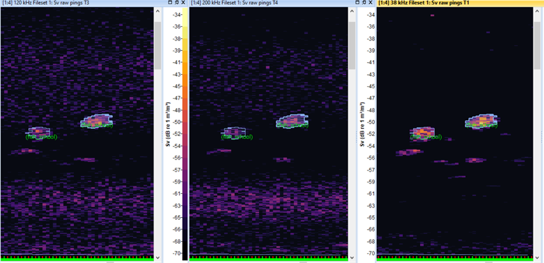
Echograms are two‑dimensional plots of acoustic echo intensity versus time and depth, in this case recorded by an echosounder – a type of marine sonar instrument that is used in oceanography to measure and analyse the water column. The goal of analysis is often to identify marine life – fish schools, plankton layers or other biological structures.

In this tutorial we build a deep‑learning pipeline for echogram segmentation using open‑source tools. We rely on PyTorch for tensor operations and GPU acceleration, PyTorch Lightning to simplify the training loop, segmentation_models_pytorch for ready‑made architectures like U‑Net. We also use xarray and Dask for handling large Zarr datasets, and scikit‑learn for data splitting and utilities.

If you'd like to jump straight into the code, you can find the notebook on Github:

The original notebook is part of a project were the main objective was to detect fish schools in hydroacoustic data, using an Atlantic herring dataset collected by NOAA Fisheries, but we tried to generalise the code so you can adapt it to your own data by setting a few configuration variables. You can find more details about the project here:

Semantic segmentation assigns a class label to every pixel, producing a mask that delineates fish from background. It differs from whole‑image classification (which produces a single label) and object detection (which outputs bounding boxes). Because fish schools form continuous, irregularly shaped regions that extend across many pings and depth bins, segmentation is the natural choice: pixel‑level labelling captures the morphology of aggregations and allows us to measure their extent, shape and height above the seafloor. Bounding boxes would either clip these shapes or include large volumes of water, while per‑image classification would completely ignore local patterns.

Data and Pre‑processing

Acoustic data in Zarr format

The data we used was recorded using a Simrad EK60 split-beam echosounder – which is a type of sonar instrument commonly used in marine studies that integrate hydroacoustic measurements. Echosounders work by recording backscatter intensity at multiple depths and frequencies.

For efficient access, the raw data are converted to a standardised format (SONAR‑netCDF4) and saved as Zarr using the echopype library – the leading open-source Python tool for hydroacoustic data processing. The Zarr format organises N‑dimensional arrays in a cloud‑optimised layout. Each ping (time sample) is indexed along a ping_time dimension, and the depth dimension is labelledrange_sample. We use the xarray library to lazily load Zarr datasets and Dask to handle out‑of‑core computation.

The notebook defines a DATA_BASE_DIR pointing at the root directory containing all data:

DATA_BASE_DIR = '/path/to/data'

# Derived directories
EVR_DIR         = os.path.join(DATA_BASE_DIR, 'EVR_region_files')
ZARR_DIR        = os.path.join(DATA_BASE_DIR, 'processed')
IMG_DIR         = os.path.join(DATA_BASE_DIR, 'ML_data', 'imgs')
MASK_DIR        = os.path.join(DATA_BASE_DIR, 'ML_data', 'masks')
BINARY_MASK_DIR = os.path.join(DATA_BASE_DIR, 'ML_data', 'binary_masks')

# Output directory for models and logs
OUTPUT_BASE_DIR = './outputs'

Loading and normalising data

We load the Zarr data lazily using xr.open_zarr so that only the necessary chunks are pulled into memory. A helper function load_combine_process_zarrs concatenates multiple Zarr files along the time dimension, sorts them chronologically, selects the first three frequency channels, drops empty pings and normalises the depth coordinate using a calibration offset.

Because the raw Sv values contain many NaNs (pings with no data), we define fill_na_with_interpolation to linearly interpolate missing values along the time axis for each channel.

After loading the dataset, we normalise each channel independently. We replace missing values with the minimum observed value minus a small offset and then linearly scale each channel to the range [0, 1]. This ensures that all channels contribute equally to the model and prevents extreme outliers from dominating the loss.

Adding the annotations

Annotations were produced by experts in fisheries acoustics in the Echoview software, the most popular software desktop tool for hydroacoustic analysis. Echoview allows a user to delineate schools and other features directly on an echogram and export the definitions to a 2D region file with the extension .evr. Each EVR file is a plain‑text record of the annotated regions, in our case for fish aggregations.

The echoregions Python library reads and writes EVR files and other Echoview formats. It supplies parsers and tools for working with EVR, EVL and ECS files and is designed to interoperate with echopype.

In our notebook we read all EVR files for a given day with a concise list comprehension:

regions2d_list = [er.read_evr(evr_file) for evr_file in evr_paths]

Because our goal is binary segmentation (fish vs. background), the annotations are converted into binary masks. The mask_class mapping is kept in a small CSV file and merged with region identifiers during mask generation.

Chunking into images and masks

Echosounder data can span many hours, producing thousands of pings. To train on manageable image sizes we cut the data into overlapping windows. The function chunk_mask takes a dataset, a list of region annotations, and a date string, then processes the data as follows:

It determines a window size equal to 1.5 × depth so that each chunk contains enough context along the vertical dimension. This preserves the aspect ratio of the data and ensures that fish schools, which may extend across many pings, are not arbitrarily split across patch boundaries.
For each window it overlays the EVR annotations to create a mask with class labels (region identifiers). Region identifiers are mapped to class indices using the region‑class table. The mask is binarised by setting all non‑zero values to 1.
If a window contains at least a minimum number of annotated pixels (by default 10), it saves the normalised image patch, the binarised mask, and the multi‑class mask as *.npy files in IMG_DIR, BINARY_MASK_DIR and MASK_DIRrespectively.

We do this to increase the number of training examples and ensure that the model sees a variety of spatial patterns.

Dataset Splitting and Augmentation

We use scikit‑learn’s train_test_split to partition the data by day into training, validation and test sets. Partitioning by day prevents information leakage between neighbouring pings, which would artificially inflate performance.

A typical split might reserve 10 % of the days for testing and 20 % of the remaining days for validation:

files = [f for f in os.listdir(IMG_DIR) if f.endswith('.npy')]
days  = list(set([f.split('_')[0] for f in files]))
train_days, test_days = train_test_split(days, test_size=0.1, random_state=1)
train_days, val_days  = train_test_split(train_days, test_size=0.2, random_state=1)

train_images = [os.path.join(IMG_DIR, f) for f in files if f.split('_')[0] in train_days]
train_masks  = [os.path.join(BINARY_MASK_DIR, f) for f in files if f.split('_')[0] in train_days]

We then define a custom SonarDataset class derived fromtorch.utils.data.Dataset. This class loads the NumPy arrays for each image and mask, applies random data augmentations (horizontal flips, random cropping and resizing to 512×512 pixels), and converts them to PyTorch tensors.

Data augmentation increases robustness by exposing the model to rotated and shifted versions of the same underlying pattern.

Model Architecture

U‑Net with a pretrained encoder

For the segmentation network we use the U‑Net architecture. U‑Net consists of a contracting path that progressively reduces spatial dimensions while capturing context and a symmetric expanding path that upsamples feature maps to produce pixel‑level predictions.

Skip connections combine local detail with global context, which is essential for capturing the elongated shapes of fish schools.

We implement U‑Net using the segmentation_models_pytorch library and choose a ResNet34 encoder pretrained on ImageNet. Pretraining provides strong low‑level feature extractors and accelerates convergence on our smaller acoustic dataset.

The network outputs a single channel per pixel, which is passed through a sigmoid activation to produce probabilities in [0, 1]. At inference time we threshold the probabilities (e.g. 0.5) to produce a binary segmentation mask.

Focal Loss for class imbalance

The dataset contains far more background than fish. If we use a standard cross‑entropy loss, the network quickly learns to predict zeros everywhere, which yields high overall accuracy but poor detection of fish schools.

Focal Loss addresses this problem by down‑weighting well‑classified examples and focusing learning on the hard examples. The loss function introduces two parameters, γ (gamma) and α (alpha), which control the strength of the focusing and the balance between classes:

class FocalLoss(nn.Module):
    def __init__(self, alpha=0.25, gamma=2.0, reduction='mean'):
        super().__init__()
        self.alpha = alpha
        self.gamma = gamma
        self.reduction = reduction

    def forward(self, inputs, targets):
        # Compute binary cross‑entropy
        bce_loss = F.binary_cross_entropy_with_logits(inputs, targets, reduction='none')
        # Compute p_t
        p_t = torch.exp(-bce_loss)
        # Compute Focal Loss
        loss = self.alpha * (1 - p_t) ** self.gamma * bce_loss
        return loss.mean() if self.reduction == 'mean' else loss.sum()

In the notebook we instantiate FocalLoss(alpha=0.25, gamma=2.0) and pass it to the Lightning module.

Evaluation Metrics

Evaluating segmentation requires more than classification accuracy because the classes are highly imbalanced. We monitor:

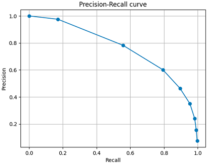
Precision (positive predictive value) and Recall (sensitivity). Precision measures the fraction of predicted pixels that are correct, while recall measures the fraction of true fish pixels that were detected.
F1 score, the harmonic mean of precision and recall.
Mean Intersection over Union (IoU), also called the Jaccard index. IoU measures the ratio of the area of overlap between the predicted segmentation and the ground truth to the area of their union. For multiple classes we compute the IoU for each class and average them.
Dice coefficient (equivalent to the F1 score for binary segmentation) and AUROC.

PyTorch Lightning integrates these metrics via the torchmetrics library.

Training Pipeline

The training pipeline is implemented using PyTorch Lightning to reduce boilerplate and handle training loops, logging and checkpointing. We define a SegModel class that inherits from pl.LightningModule and encapsulates the model, loss function, metrics and optimisers. Key methods include:

forward(x): passes the input through the U‑Net and applies sigmoid activation.
training_step/validation_step/test_step: compute predictions, apply loss, update metrics and return the loss for backpropagation.
configure_optimizers(): constructs the optimiser (Adam) and learning rate scheduler.
on_test_epoch_end(): generates a confusion‑matrix plot and logs aggregated metrics to the logger.

We instantiate the model with a chosen encoder and loss function:

encoder_name = 'resnet34'
encoder_weights = 'imagenet'
model = smp.Unet(
    encoder_name=encoder_name,
    encoder_weights=encoder_weights,
    in_channels=3,
    classes=1,
    activation=None
)
criterion = FocalLoss(alpha=0.25, gamma=2.0)
optimizer = torch.optim.Adam(model.parameters(), lr=1e-4)
pl_model = SegModel(model, criterion, optimizer)

To train the model we create data loaders with appropriate batch sizes and the number of worker processes equal to the number of CPU cores:

train_loader = DataLoader(train_dataset, batch_size=4, shuffle=True,  num_workers=os.cpu_count(), pin_memory=True)
val_loader   = DataLoader(val_dataset,   batch_size=4, shuffle=False, num_workers=os.cpu_count(), pin_memory=True)

We then configure the Trainer:

logger = TensorBoardLogger(
    save_dir=os.path.join(OUTPUT_BASE_DIR, 'tb_logs'),
    name=run_name
)

checkpoint = ModelCheckpoint(
    dirpath=os.path.join(OUTPUT_BASE_DIR, 'checkpoints'),
    monitor='val_f1',
    mode='max',
    save_top_k=3
)
early_stopping = EarlyStopping(monitor='val_f1', mode='max', patience=10)
lr_monitor = LearningRateMonitor()

trainer = pl.Trainer(
    accelerator='auto', devices=1,
    precision='16-mixed',  # Use mixed precision for faster training
    max_epochs=100,
    logger=logger,
    callbacks=[checkpoint, early_stopping, lr_monitor]
)
trainer.fit(pl_model, train_loader, val_loader)

Setting accelerator='auto' allows Lightning to pick the appropriate device (GPU if available). The precision='16-mixed' flag enables automatic mixed precision for faster training on modern GPUs while preserving numerical stability.

Results over 10 cross val runs (prob. threshold 0.5)

After training completes, you can evaluate the model on the test set:

test_loader = DataLoader(test_dataset, batch_size=4, shuffle=False, num_workers=os.cpu_count(), pin_memory=True)
trainer.test(pl_model, dataloaders=test_loader)

GPU and device configuration

Training is of course most efficient when performed on a graphics processing unit (GPU) and in our notebook we detect whether a CUDA‑enabled device is available and set a device variable accordingly:

device = 'cuda' if torch.cuda.is_available() else 'cpu'

All input tensors and the model itself are moved onto this device before training. When configuring the PyTorch Lightning Trainer we set accelerator='auto'and devices=1 so that Lightning chooses a GPU when present and falls back to the CPU otherwise.

The option precision='16-mixed' enables automatic mixed‑precision training, which stores activations in 16‑bit floats and accumulates gradients in 32‑bit precision. This reduces memory consumption and can accelerate training on modern GPUs without degrading accuracy.

On a mid‑range GPU such as an NVIDIA RTX 3060 with at least 12 GB of memory, training this U‑Net model with a batch size of four completes in a few hours. On CPU‑only systems the same experiment may take days, so you may need to reduce the batch size to fit into RAM. On multi‑GPU workstations you can set devices to the number of available GPUs to train in parallel.

Conclusion

This tutorial walked through the end‑to‑end process of preparing acoustic data, building a segmentation dataset, training a U‑Net model with a pretrained encoder, using Focal Loss to mitigate class imbalance, and evaluating performance. Our goal was to abstract hyperparameters into configuration variables so that the notebook becomes portable and adaptable to new datasets.

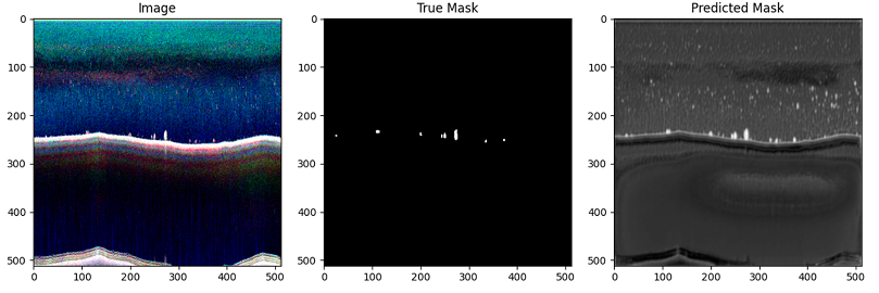
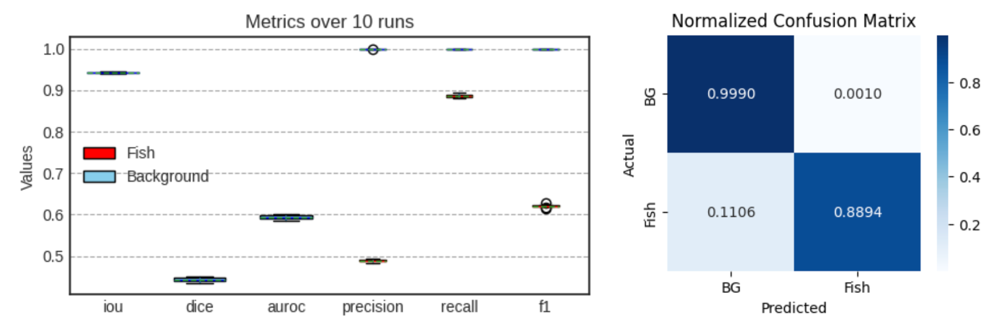
In our experiment, we started with a small dataset – 18 days of observations. These data have been manually annotated by experts outlining the regions which they believed to be fish schools. Even with this modest amount of training data, our model managed to detect 90% of the pixels the researchers marked as fish, however, it was a bit too eager, with about 50% of the pixels it marked actually matching what the humans had identified.