Using Copernicus Satellite Observations to Improve Ocean Acoustic Measurements

Introduction

Hydroacoustic instruments are important tools for observing the ocean. These systems measure sound echoes to map the seafloor, estimate the marine life abundance and biomass, and characterise water‑column processes. The accuracy of such measurements depends fundamentally on our knowledge of how sound propagates through seawater.

This article outlines how we retrieve Copernicus Marine Service data and compute sound speed profiles (SSPs) using Python.

If you want to dive straight into the code, the workflow is available as a Jupyter notebook on Github:

sound-speed-profile/SSP_from_Copernicus.ipynb at main · OceanStreamIO/sound-speed-profile

Contribute to OceanStreamIO/sound-speed-profile development by creating an account on GitHub.

GitHubOceanStreamIO

Using sound speed profiles in hydroacoustics

Echosounders work by emitting acoustic pulses and recording the echoes as discrete time‑sampled signals. To convert these samples into ranges and then into volume backscattering strength (Sv), two key parameters are required: the speed of sound and the absorption coefficient. 

Sound travels faster or slower depending on temperature, salinity and pressure, so an accurate sound speed profile (SSP) and absorption coefficient of seawater are essential for converting raw echosounder signals into meaningful depths and calibrated backscattering strengths.

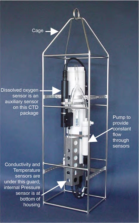
In practice, CTD sensors (conductivity, temperature, and depth) are used to derive SSPs and to provide the gold-standard truth used at sea and in post-processing. The CTD is an essential tool used in all disciplines of oceanography, providing important information about physical, chemical, and even biological properties of the water column.

Ocean Physics – sound propagation in seawater

In seawater the speed of sound is controlled principally by temperature, salinity and pressure. It increases with warmth, salinity, and depth (pressure), and decreases in colder or fresher water.

Empirical measurements show that sound speed typically ranges from about 1 450 to 1 570 m s⁻¹ and increases roughly by 4.5 m s⁻¹ per degree Celsius, 1.3 m s⁻¹ per practical salinity unit and 1.7 m s⁻¹ per decibar of pressure (National Physical Laboratory, 2000). These sensitivities mean that errors of only a few degrees or salinity units can introduce several metres of range error for sonar soundings hundreds of metres deep.

Several formulae have been developed to compute the sound speed from environmental parameters. A widely used empirical relation is the nine‑term Mackenzie equation, which expresses sound speed c in metres per second as a function of temperature T (°C), salinity S (PSU) and depth D (m):

This equation is valid for temperatures 2–30 °C, salinities 25–40 PSU and depths up to 8 000 m. It has been used extensively because of its simplicity and good accuracy in the typical open‑ocean range. Modern thermodynamic standards, such as the Thermodynamic Equation of Seawater 2010 (TEOS‑10), use a 75‑term polynomial to compute sound speed from absolute salinity, conservative temperature and sea pressure. The gsw Python library, part of the TEOS‑10 toolset, implements this expression and is considered more accurate, particularly in extreme salinity or pressure conditions.

Copernicus Marine Environment Monitoring Service (CMEMS)

In recent years satellite model‑based Earth‑observation programmes have made it possible to derive environmental parameters of the ocean at high spatial and temporal resolution. The European Union’s Copernicus programme provides free and open access to global datasets on the physical, biogeochemical and sea‑ice state of the ocean.

Through the Copernicus Marine Environment Monitoring Service (CMEMS), users can obtain regular reference information on variables such as sea‑water salinity (PSU) and potential temperature for the global ocean and regional seas.

In this article, we describe a methodology for deriving SSPs from Copernicus satellite observations in order to improve the calibration of echosounder data, particularly when CTD measurements are sparse or unavailable.

Copernicus is the European Union’s flagship Earth‑observation programme, overseen by the European Commission in partnership with the European Space Agency (ESA), the European Organisation for the Exploitation of Meteorological Satellites (EUMETSAT), the European Centre for Medium‑Range Weather Forecasts (ECMWF) and several national agencies. The programme operates a family of dedicated satellites (the Sentinel series) and provides data from contributing missions and in situ networks. All Copernicus services are free, open and designed to benefit the society.

The Copernicus Marine Environment Monitoring Service delivers regular and systematic information on the state of the global ocean and European seas. It assimilates satellite observations and in situ measurements into numerical ocean models to produce near‑real‑time and forecast fields of different marine variables.

These variables are divided into three categories:

• the blue ocean monitors the physical state of the ocean,
• the green ocean monitors the biogeochemical parameters,
• the white ocean monitors sea ice.

Datasets used

Datasets are provided at resolutions down to 0.083° (≈8 km) with daily or even hourly temporal sampling.

In our project we use the CMEMS  GLOBAL_ANALYSISFORECAST_PHY_001_024 product (system name GLO12) which delivers global ocean physical fields at 1/12° (~0.083°) with analysis and forecast components. The current data store organises variables into granular dataset IDs, e.g. cmems_mod_glo_phy–so_anfc_0.083deg_P1D‑m and cmems_mod_glo_phy–thetao_anfc_0.083deg_P1D‑m which supply three‑dimensional fields of practical salinity and seawater potential temperature respectively (daily means) for the full water column.

Integrating SSPs into sonar data processing

In our data processing pipelines, we use the open‑source echopype library which accepts environmental parameters—temperature, salinity, pressure and pH—to compute sound speed and absorption via empirical formulae. The sound speed controls the range conversion (echo_range) from sample index and sample interval, while the absorption coefficients determine the attenuation correction for spherical spreading and seawater absorption.

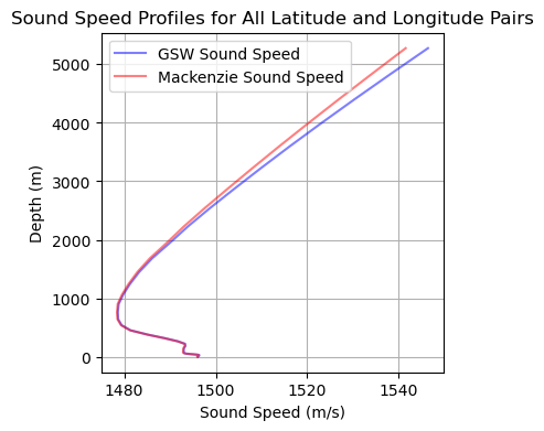
The difference between TEOS‑10 and Mackenzie sound speed in the figure above illustrates sensitivity of accurate SSPs. Near the surface, where temperatures are high and salinities are relatively low, the Mackenzie formula underestimates the sound speed by ~1–2 m s⁻¹ compared with TEOS‑10. At greater depths (>1 000 m) the divergence grows because the Mackenzie formula approximates pressure dependence by depth, whereas TEOS‑10 uses pressure and absolute salinity; differences of 3–4 m s⁻¹ emerge.

Deriving sound speed profiles from Copernicus data

Below we outline how to retrieve Copernicus Marine Service data and compute SSPs using Python. The workflow is implemented in a Jupyter notebook SSP_from_Copernicus.ipynb.

Here's the complete workflow:

1. Specify the target location and time window;
2. Retrieve salinity and potential temperature fields – result is an xarray dataset with dimensions depth, latitude and longitude;
3. Compute sound speed using TEOS‑10
4. Compute sound speed using the Mackenzie formula
5. Transform the data and visualise

Here's an excerpt from the Python code used to compute the SSP. The full code is available in the notebook.

import xarray as xr
import copernicusmarine
import gsw
from datetime import datetime, timedelta

# Define location and time window
target_lon, target_lat = -170.2, 40.4
days_back = 10
end_time = datetime.utcnow()
start_time = end_time - timedelta(days=days_back)

# Open salinity and potential temperature datasets
sal_ds = copernicusmarine.open_dataset(dataset_id='cmems_mod_glo_phy-so_anfc_0.083deg_P1D-m',
    minimum_longitude=target_lon, maximum_longitude=target_lon,
    minimum_latitude=target_lat, maximum_latitude=target_lat,
    start_datetime=start_time, end_datetime=end_time, variables=['sea_water_salinity'])

temp_ds = copernicusmarine.open_dataset(dataset_id='cmems_mod_glo_phy-thetao_anfc_0.083deg_P1D-m',
    minimum_longitude=target_lon, maximum_longitude=target_lon,
    minimum_latitude=target_lat, maximum_latitude=target_lat,
    start_datetime=start_time, end_datetime=end_time, variables=['sea_water_potential_temperature'])

# Merge salinity and temperature datasets
measurement_ds = xr.merge([sal_ds, temp_ds])

# Compute sound speed with TEOS‑10
SA = gsw.SA_from_SP(measurement_ds['so'], gsw.p_from_z(-measurement_ds['depth'], measurement_ds['latitude']), measurement_ds['longitude'])
CT = gsw.CT_from_pt(SA, measurement_ds['thetao'])
p  = gsw.p_from_z(-measurement_ds['depth'], measurement_ds['latitude'])
measurement_ds['GSW_sound_speed'] = gsw.sound_speed(SA, CT, p)

# Compute sound speed with Mackenzie
def mackenzie(temp, sal, depth):
    return (1448.96 + 4.591*temp - 5.304e-2*temp**2 + 2.374e-4*temp**3 +
            1.34*(sal - 35) + 1.63e-2*depth + 1.675e-7*depth**2 - 1.025e-2*temp*(sal - 35) - 7.139e-13*temp*depth**3)

measurement_ds['Mackenzie_sound_speed'] = mackenzie(measurement_ds['thetao'], measurement_ds['so'], measurement_ds['depth'])

Computing SSPs at the Edge

OceanStream provides a flexible architecture for deploying these workflows on IoT Edge devices, enabling real‑time oceanographic processing in remote marine environments. The IoT Edge architecture pushes computing to the point of data collection while maintaining connectivity to powerful cloud resources. 

Internet‑of‑Things (IoT) platforms typically focus on collecting sensor readings and streaming them to the cloud for analysis. In contrast, edge computing refers to executing computational workloads on or near the sensors themselves, thereby reducing the latency and bandwidth required to transmit raw data. 

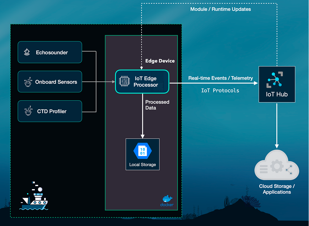
Copernicus data retrieval provides a viable way to forecast the SSPs ahead of the mission and the data can be deployed on the Edge device to be used as needed, when connectivity is intermittent and when CTD sensors aren't available.

Edge compute is invaluable when bandwidth is constrained or when operators need immediate feedback to adjust instrument settings (pulse lengths, ping rates) or survey patterns. 

Conclusion

The Copernicus programme provides free and open data which can be used to derive temperature and salinity profiles anywhere in the global ocean and compute SSPs using well‑established physical relationships, which can be integrated into hydroacoustic measurements for meaningful oceanographic information.

The example presented here demonstrates how remote observations can be combined with the TEOS‑10 and Mackenzie equations to generate SSPs in Python. Integrating such SSPs into our workflows improves the calibration of volume backscattering strength (Sv), in order to improve the biomass estimates and physical interpretations of the water column.

Authors: Andrei Rusu, Katja Ovchinnikova, Tomos David