
Introduction
The OceanStream Globe is a new ocean data service we are building as part of the OceanStream platform. It is continuously downloading and processing daily physics and biogeochemistry data for the global ocean, computing historical time series and per-pixel statistics, and displaying the results on a rotating 3D globe.
Data comes mainly from Copernicus Marine Service (CMEMS) and each dataset is represented as a grid over the ocean. For every grid cell the Globe holds long-term statistics, such as the average and the usual range, so that any location can be compared with its own normal. This article describes the sea-surface temperature (SST) workflows and how we can use the service to inspect El Niño – the recurring ocean-atmosphere climate pattern in the tropical Pacific, which is now under way.
OceanStream Globe runs on EDITO DataLab, the core infrastructure of the European Digital Twin Ocean, and uses the MareNostrum 5 supercomputer in Barcelona via the EuroHPC JU programme for batch processing jobs.
What is El Nino?
El Niño is the warm phase of the El Niño–Southern Oscillation (ENSO), a natural swing in tropical Pacific sea temperatures and winds that recurs every 3–7 years on average; La Niña is the cold phase (Explaining El Niño). Its effects reach well beyond the Pacific. El Niño years have brought heavier rain to the southern United States and to Peru, and drought to the western Pacific, at times with severe bushfires in Australia.
Measurements from the tropical Pacific are a key input to climate forecasts from a few months to a year ahead. The necessary data is provided through the Tropical Pacific Observing System (TPOS), an international collaboration that combines data from moored buoys and other ocean platforms, research ships, and satellite measurements of sea-surface temperature, winds and sea level (TPOS).
Satellites map sea-surface temperature across the whole basin every day. The dataset used in this article is a gap-filled analysis built from them, called OSTIA (Operational Sea Surface Temperature and Sea Ice Analysis), produced by the UK Met Office and distributed by the Copernicus Marine Service.
The SST archive
For SST, we use a 35-year global archive derived from Copernicus Marine OSTIA. The climatology covers 1991–2020, while the observation record continues through September 2026.
An SST anomaly is the difference between an observation and a reference value. For this service we use the 1991–2020 World Meteorological Organization (WMO) standard reference period. Thirty years provides a baseline spanning several ENSO (El Niño–Southern Oscillation) cycles and makes the resulting anomalies easier to compare with products using the same period.
Copernicus Marine OSTIA L4 is a daily, global foundation sea-surface-temperature analysis on a 0.05° grid (about 5.5 km north–south, with east–west spacing narrowing towards the poles). Foundation SST represents temperature without the daily surface-warming cycle. The analysis fills gaps between observations, giving us a consistent ocean grid for historical comparisons. Land and invalid values are masked, and statistics use the valid observations available at each pixel.
We combine two Copernicus Marine products:
| Stream | Dataset | Coverage used |
|---|---|---|
| Reprocessed | METOFFICE-GLO-SST-L4-REP-OBS-SST | From 1991-01-01 |
| Near-real-time | METOFFICE-GLO-SST-L4-NRT-OBS-SST-V2 | Latest period to present |
They overlap by 805 days, counting both endpoints, so there is no gap to bridge. The overlap allows a choice of handover date. We start at 1991-01-01 because that is where the WMO window begins, giving 13,034 daily fields through 2026-09-07.
Each day is converted to a Cloud-Optimised GeoTIFF, int16 with a 0.01 °C encoding increment and land masked out. That increment describes storage precision, not the accuracy of the SST analysis. Compressed file sizes vary with the field; the expanded data volume is the useful measure for the reduction.
We ingested the daily OSTIA record from 1991 and computed the climatology over the full 1991–2020 window. The baseline contains 10,958 daily fields.
The Pacific, with and without a baseline
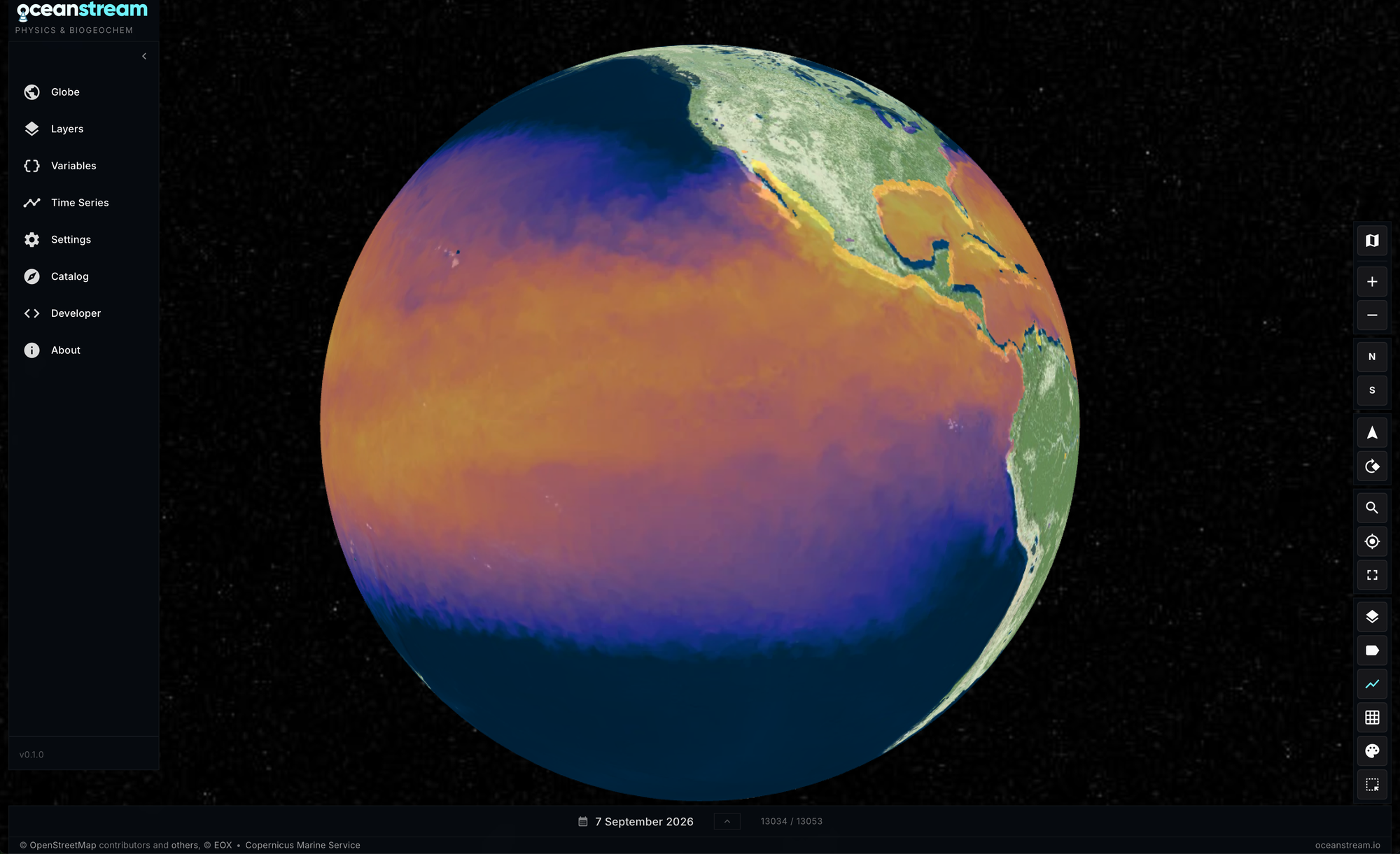
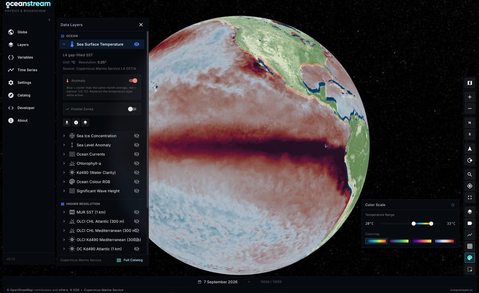
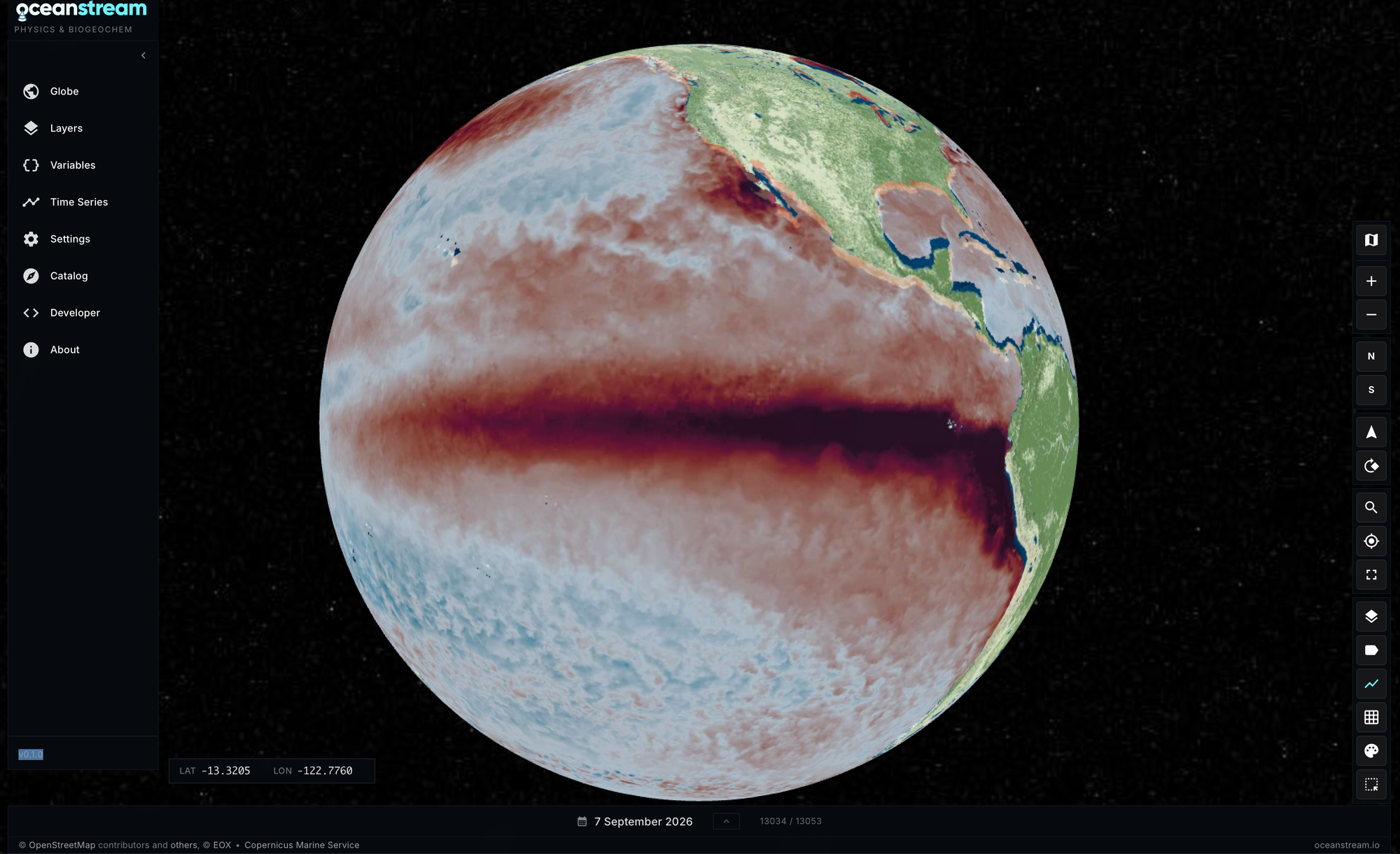
Absolute sea-surface temperature across the tropical Pacific on 7 September 2026 and anomaly for the same day, relative to the 1991–2020 climatology. The equatorial warm tongue is immediately visible. The colour scale is 20-33 °C.
The absolute SST field shows how warm the water is, but it does not directly show the departure from usual conditions. Much of the broad warm band around the equator reflects the normal temperature structure of the tropical Pacific.
Subtracting the 1991–2020 average for that time of year makes the anomalous structure much clearer. A strong positive anomaly extends along the equatorial Pacific towards South America, with the largest values in the eastern basin.
The absolute map is not wrong; it answers a different question. Absolute SST tells us how warm the water is. The anomaly tells us how unusual it is relative to a stated reference period.
Parts of the central and eastern equatorial Pacific are several degrees above the September average, locally exceeding +5 °C. For example, near 0°, 100°W, the API returns an SST of 27.17 °C and a September climatology of 21.57 °C, a difference of about +5.6 °C.
Computing the climatology on MareNostrum 5
For every ocean pixel we need to reduce the complete baseline period, and for some statistics we need the full temporal distribution. For each of the 3600 × 7200 grid cells we compute the 1991–2020 average, spread and 10th, 50th and 90th percentiles, for the whole year and for each calendar month, plus a linear trend over the full 1991–2026 record.
Across 13,034 daily fields this means passing about 1.35 TB of float32 values through the calculation. Averages and trends can be updated as each day streams in, but percentiles need a cell's whole 30-year series in memory at once: about 24.6 GiB for each 512 × 512 tile.
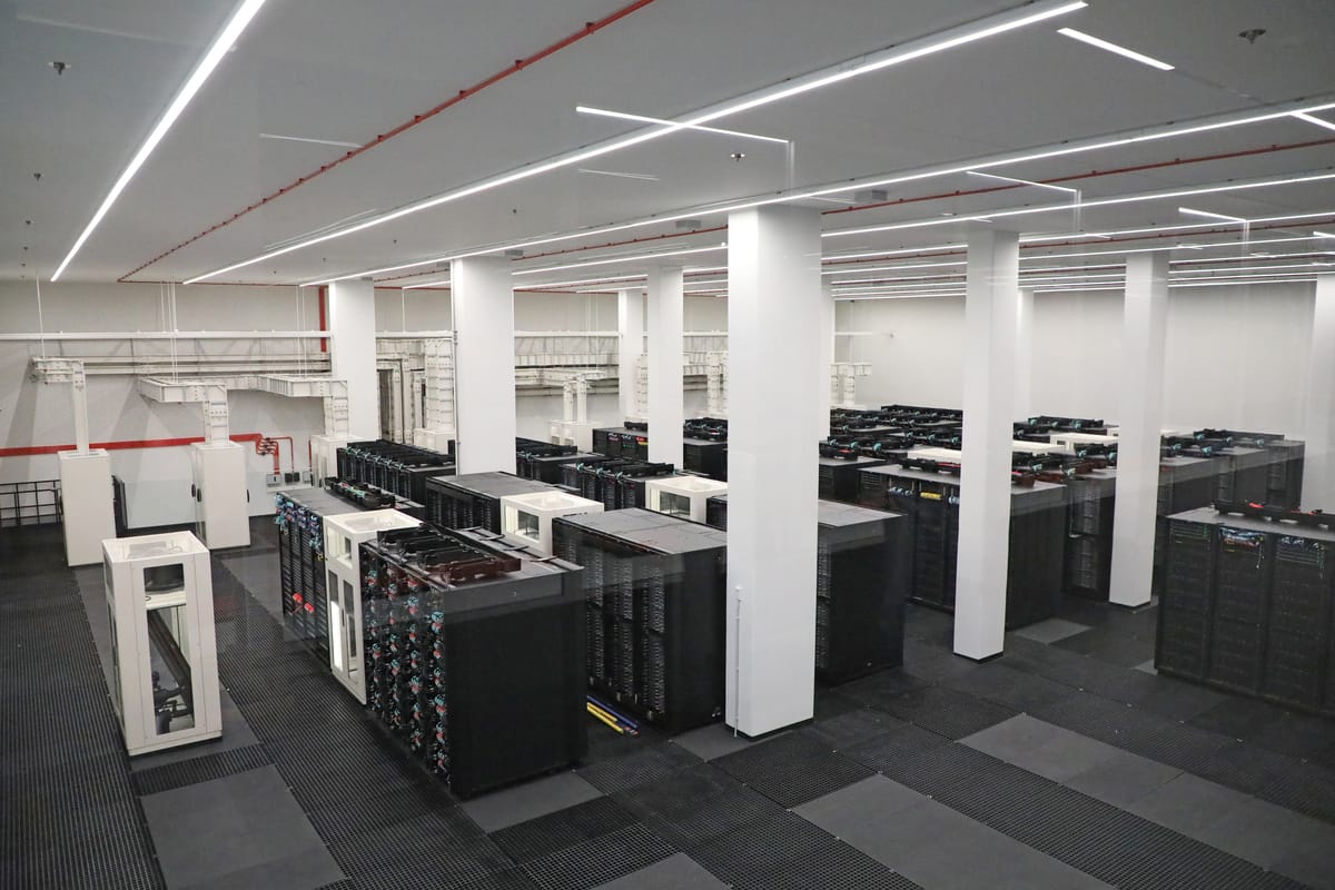
The job runs on MareNostrum 5 at the Barcelona Supercomputing Center. The full 35-year run took 2 hours 35 minutes, of which about 21 minutes was the percentile pass.
The two kinds of statistic answer different questions. The 1991–2020 values define what is normal for each cell in each calendar month, so a September day is compared with past Septembers: the anomaly map subtracts the monthly average, and the shaded band in the Time Series view is the 10th–90th percentile range.
The trend describes how each cell has changed, as a linear fit over the whole record from 1991 through 2026, including the years after the baseline. Each stored array records the period it was computed over, and the labels on the Globe come from that metadata.
Moving data between EDITO and the HPC
MareNostrum's compute nodes do not have outbound internet access. That is quite normal for HPC, but it changes the architecture. The job cannot read directly from Copernicus Marine or S3, and it cannot fetch code or install packages at runtime. Everything it needs has to be staged onto the parallel filesystem before the job starts, and the results need to leave through the transfer infrastructure afterwards.
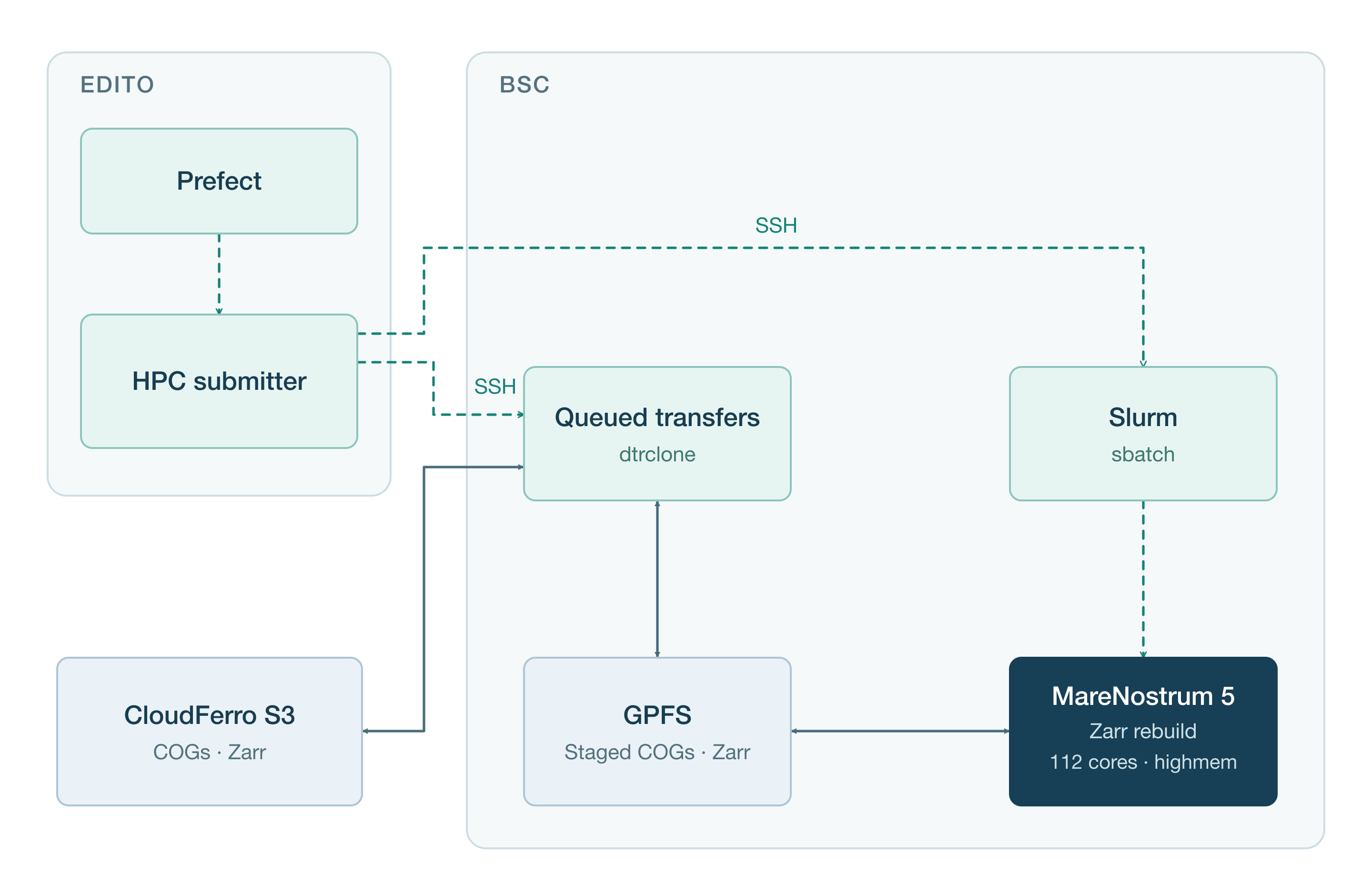
EDITO Datalab is a Kubernetes-based compute environment, and we're using it for the download, conversion and orchestration stages. The orchestration itself synchronises the processing code and submits the Slurm job (the workflow manager that the HPC uses).
Checking against NOAA Climate Prediction Center
To check the SST pipeline, we implemented the four standard Niño box indices independently and compared the weekly output with NOAA Climate Prediction Center (CPC).
The comparison follows CPC’s weekly convention and uses area weighting from exact spherical latitude strips. It covers 2021 to September 2026, outside the 1991–2020 climatology period.
| Region | RMS (°C) | Bias (°C) | Correlation |
|---|---|---|---|
| Niño 1+2 | 0.291 | −0.016 | 0.983 |
| Niño 3 | 0.127 | −0.028 | 0.994 |
| Niño 3.4 | 0.101 | −0.035 | 0.995 |
| Niño 4 | 0.119 | −0.070 | 0.992 |
For Niño 3.4 the agreement is particularly close: 0.10 °C RMS with a correlation of 0.995. The products use different SST analyses: CPC uses NOAA OISST, while our calculation uses Copernicus Marine OSTIA.
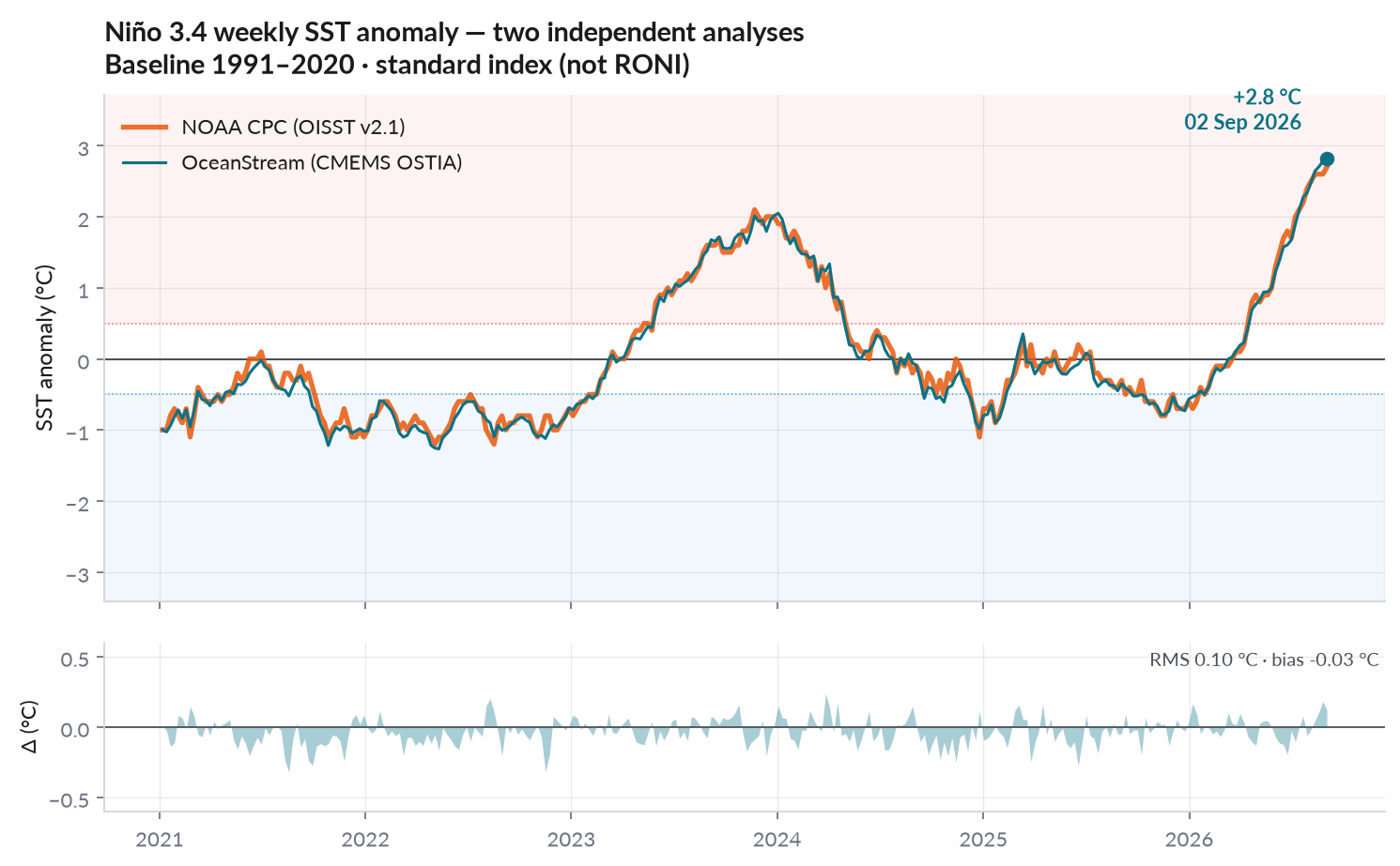
The residual panel shows where the products diverge. Through the 2021–2023 La Niña, the 2023–2024 El Niño and the sharp rise in 2026, the two lines generally sit on top of each other.
The 2026 event across the four Niño regions
The four regions are useful because they show how the event is distributed from the South American coast towards the central Pacific. By early September 2026, the strongest anomaly in our weekly series is in Niño 1+2, at about +4.8 °C. Niño 3 is around +3.7 °C, Niño 3.4 around +2.8 °C, and Niño 4 about +1.0 °C.
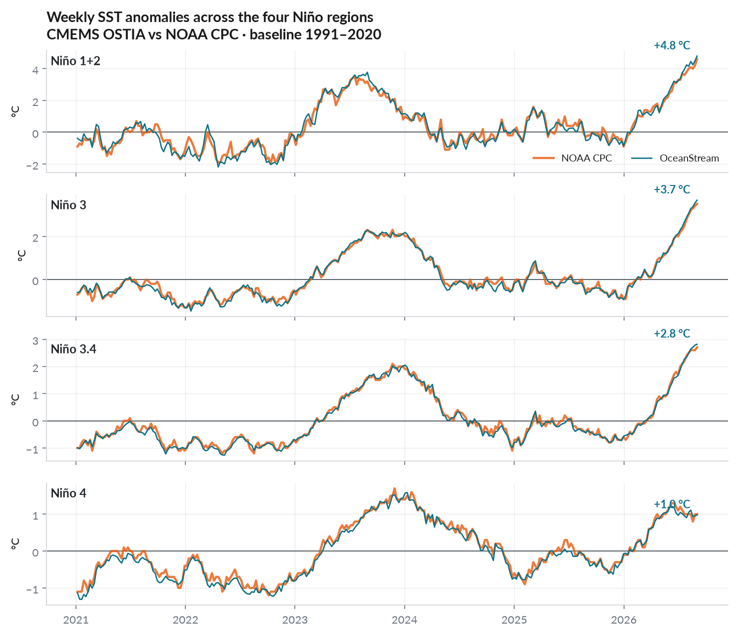
This east-to-west gradient is also visible in the anomaly map. What we wanted was an independently derived index that lets us validate the OceanStream climatology and then connect the same numbers to the global map and per-pixel time series.
European infrastructure from data to compute
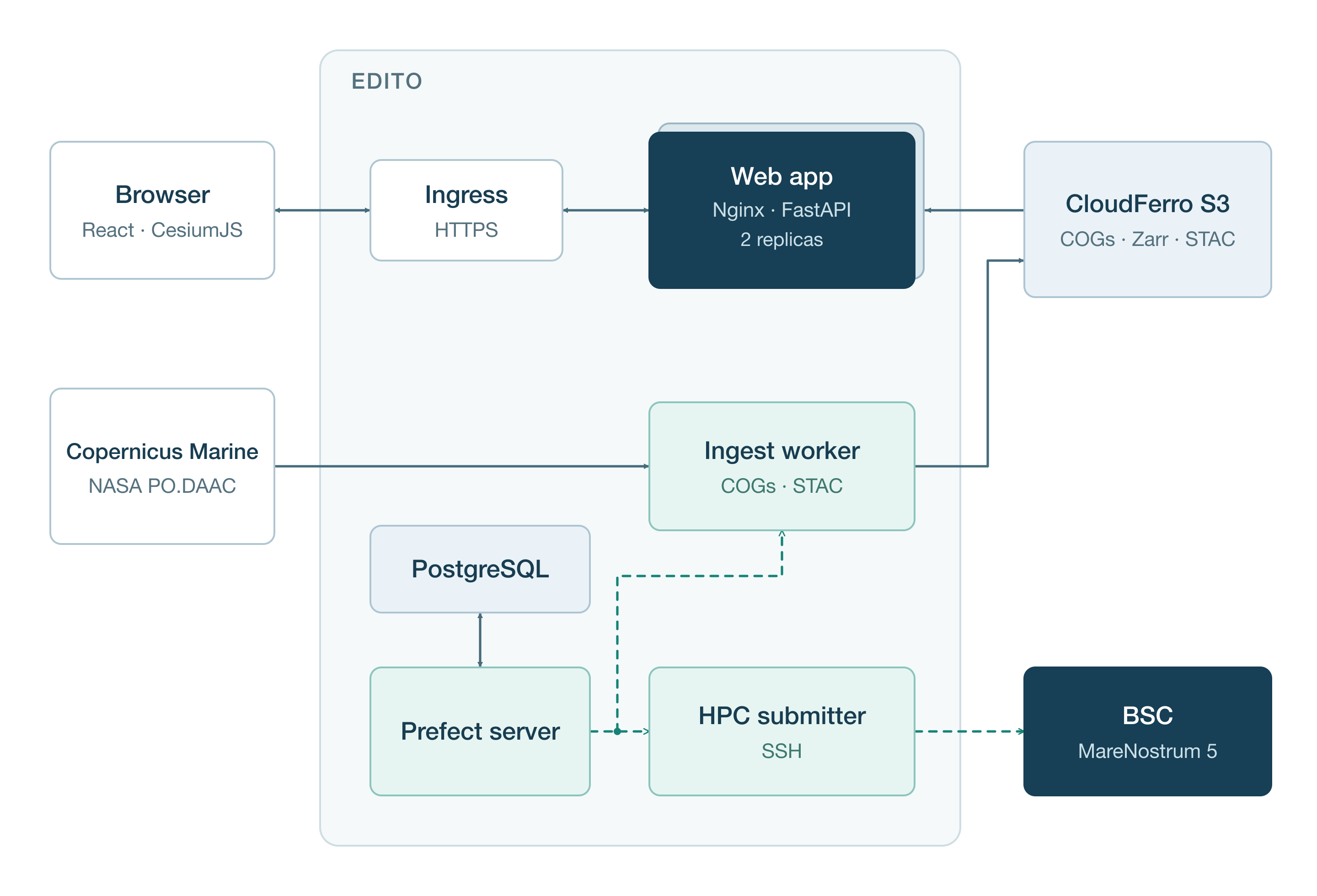
EDITO is the European public cloud platform for ocean data applications, models, and datasets, under the European Digital Twin Ocean initiative. It's developed in Toulouse by Mercator Ocean International (same organisation that maintains CMEMS) and the cloud compute infrastructure is operated by CloudFerro, in Warsaw (a Polish company is part of the consortium hosting the Copernicus Data Ecosystem Services, among others)
MareNostrum 5 is operated at the Barcelona Supercomputing Center – a public research center, and it's available via the EuroHPC-JU programme.
Therefore, the complete pipeline runs on European infrastructure, from start to end:
- Data: Copernicus Marine Service OSTIA
- Platform: EDITO Datalab / European Digital Twin Ocean
- Storage: CloudFerro
- Batch processing: MareNostrum 5 through EuroHPC
We can start with operational Earth-observation data, run orchestration in Kubernetes, stage the inputs through object storage and carry out a high-memory reduction on a EuroHPC system.
Try it
The OceanStream Globe web app is live at https://globe.oceanstream.io, in public preview. Give it a try: open the Layers panel, select SST, and toggle the Anomaly button. Click an ocean location and open Time Series. Use the globe timeline to inspect individual daily maps.
If you're interested to find out more, or you need assistance with accessing the data in our catalog, simply get in touch with us via the button below. Bug reports are always appreciated and feature requests are welcome.
Get in touch to request more information or report issues.